Table of contents

SPICE
Simulation Program with Integrated Circuit Emphasis
Find right transistor sizes
More information
Analog Design
Demo
Summary
Would you like to know more?

SPICE

Keywords: SPICE, Sources, Passives, Transistor Models, BSIM, Foundries, Unit Transistors, gm/ID

Simulation Program with Integrated Circuit Emphasis

To manufacture an integrated circuit we have to be able to predict how it’s going to work. The only way to predict is to rely on our knowledge of physics, and build models of the real world in our computers.

One simulation strategy for a model of the real world, which absolutely every single integrated circuit in the world has used to come into existence, is SPICE.

Published in 1973 by Nagel and Pederson

SPICE (Simulation Program with Integrated Circuit Emphasis)

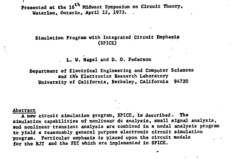
_{Figure 1: Title page of Nagel and Pederson’s 1973 SPICE paper from the 16th Midwest Symposium on Circuit Theory. Source: L. W. Nagel, SPICE2 memorandum ERL-M520, UC Berkeley, 1975}

Today

There are multiple SPICE programs that has been written, but they all work in a similar fashion. There are expensive ones, closed source, and open source.

Some are better at dealing with complex circuits, some are faster, and some are more accurate. If you don’t have money, then start with ngspice.

Commercial Cadence Spectre Siemens Eldo Synopsys HSPICE

Free Aimspice Analog Devices LTspice

Open Source ngspice

But

All SPICE simulators understand the same language (yes, even spectre can speak SPICE). We write our testbenches in a text file, and give it to the SPICE program. That’s the same for all programs. Some may have built fancy GUI’s to hide the fact that we’re really writing text files, but text files is what is under the hood.

Pretty much the same usage model as 50-odd years ago

<spice program> testbench.cir

for example

ngspice testbench.cir

Or in the most expensive analog tool (Cadence Spectre)

spectre  input.scs  +escchars +log ../psf/spectre.out 
-format psfxl -raw ../psf   +aps +lqtimeout 900 -maxw 5 
-maxn 5 -env ade  -ahdllibdir 
/tmp/wulff/virtuoso/TB_SUN_BIAS_GF130N/TB_SUN_BIAS/maestro/
results/maestro/Interactive.15/sharedData/CDS/ahdl/input.ahdlSimDB 
+logstatus 

The expensive tools have built graphical user interface around the SPICE simulator to make it easier to run multiple scenarios.

Corner	Typical	Fast	Slow	All
Mosfet	Mtt	Mff	Mss	Mff,Mfs,Msf,Mss
Resistor	Rt	Rl	Rh	Rl,Rh
Capacitors	Ct	Cl	Ch	Cl,Ch
Diode	Dt	Df	Ds	Df,Ds
Bipolar	Bt	Bf	Bs	Bf,Bs
Temperature	Tt	Th,Tl	Th,Tl	Th,Tl
Voltage	Vt	Vh,Vl	Vh,Vl	Vh,Vl

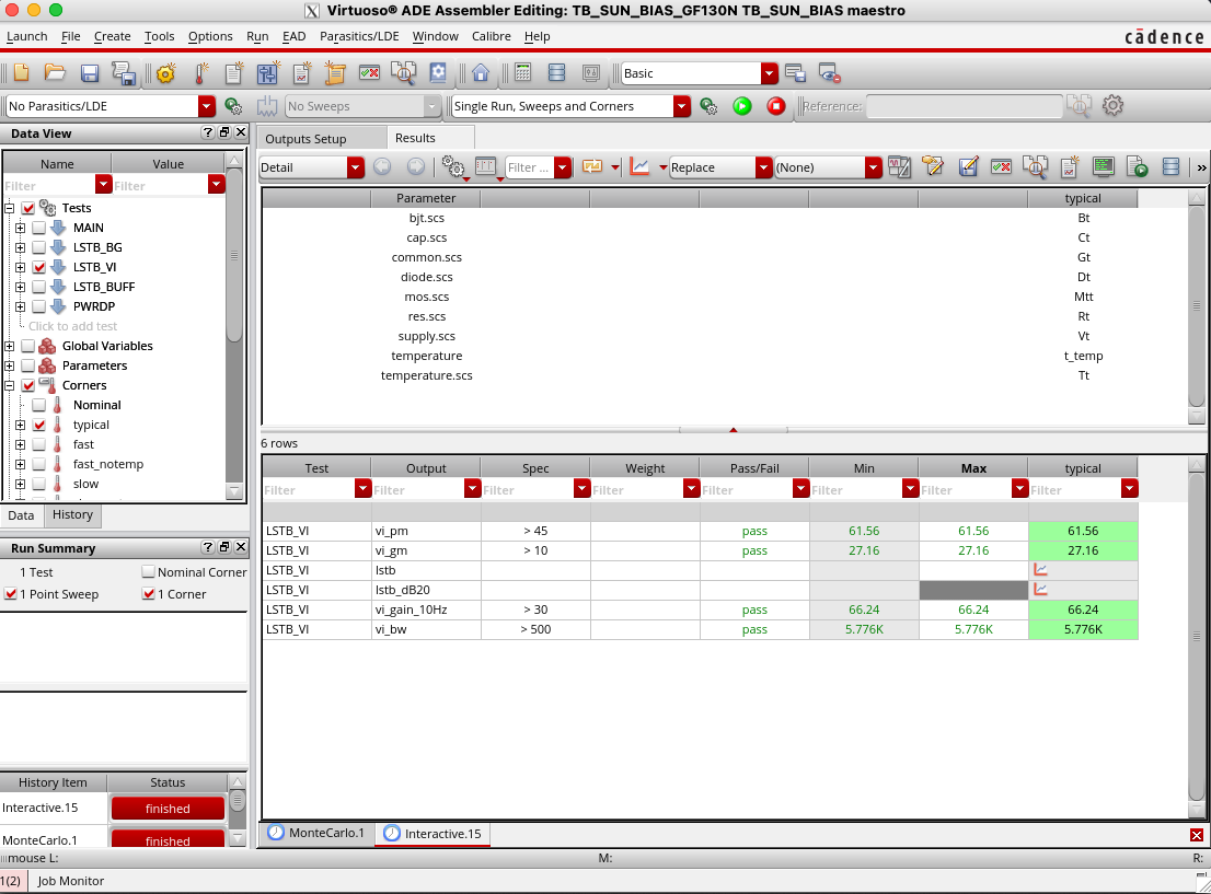
_{Figure 2: Cadence Virtuoso ADE Assembler, showing the corner definitions on the left and a pass/fail table of simulated specifications on the right}

I’m a fan of launching multiple simulations from the command line. I don’t like GUI’s. As such, I wrote cicsim, and that’s what I use in the video and demo.

Sources

The SPICE language is a set of conventions for how to write the text files. In general, it’s one line, one command (although, lines can be continued with a +).

I’m not going to go through an extensive tutorial in this document, and there are dialects with different SPICE programs. You’ll find more info at ngspice

Independent current sources

_{Infinite output impedance, changing voltage does not change current}

I<name> <from> <to> dc <number> ac <number>

I1 0 VDN dc In
I2 VDP 0 dc Ip

Independent voltage source

_{Zero output impedance, changing current does not change voltage}

V<name> <+> <-> dc <number> ac <number>

V2 VSS 0 dc 0
V1 VDD 0 dc 1.5

Passives

Resistors

R<name> <node 1> <node 2> <value>

R1 N1 N2 10k
R2 N2 N3 1Meg
R3 N3 N4 1G
R4 N4 N5 1T

Capacitors

C<name> <node 1> <node 2> <value>

C1 N1 N2 1a
C2 N1 N2 1f
C4 N1 N2 1p
C3 N1 N2 1n
C5 N1 N2 1u

Transistor Models

Needs a model file describing the transistor model

BSIM (Berkeley Short-channel IGFET Model) http://bsim.berkeley.edu/models/bsim4/

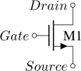
_{Figure 3: Circuit symbol for an NMOS transistor with its gate, drain and source terminals}

284 parameters in BSIM 4.5

.MODEL N1 NMOS LEVEL=14 VERSION=4.5.0 BINUNIT=1 
PARAMCHK=1 MOBMOD=0 CAPMOD=2 IGCMOD=1 IGBMOD=1 
GEOMOD=1  DIOMOD=1 RDSMOD=0 RBODYMOD=0 RGATEMOD=3
PERMOD=1 ACNQSMOD=0 TRNQSMOD=0 TEMPMOD=0  TNOM=27 
TOXE=1.8E-009 TOXP=10E-010 TOXM=1.8E-009  DTOX=8E-10 
EPSROX=3.9 WINT=5E-009 LINT=1E-009 LL=0 WL=0 LLN=1 
WLN=1  LW=0 WW=0 LWN=1 WWN=1  LWL=0 WWL=0 XPART=0
TOXREF=1.4E-009  SAREF=5E-6 SBREF=5E-6 WLOD=2E-6 
KU0=-4E-6  KVSAT=0.2 KVTH0=-2E-8 TKU0=0.0 LLODKU0=1.1  
WLODKU0=1.1 LLODVTH=1.0 WLODVTH=1.0 LKU0=1E-6  
WKU0=1E-6 PKU0=0.0 LKVTH0=1.1E-6 WKVTH0=1.1E-6  
PKVTH0=0.0 STK2=0.0 LODK2=1.0 STETA0=0.0  LODETA0=1.0  
LAMBDA=4E-10  VSAT=1.1E 005 VTL=2.0E5 XN=6.0 LC=5E-9 
RNOIA=0.577 RNOIB=0.37 LINTNOI=1E-009  WPEMOD=0 
WEB=0.0 WEC=0.0 KVTH0WE=1.0  K2WE=1.0 KU0WE=1.0 SCREF=5.0E-6
TVOFF=0.0 TVFBSDOFF=0.0  VTH0=0.25  K1=0.35 K2=0.05
K3=0  K3B=0 W0=2.5E-006 DVT0=1.8 DVT1=0.52  DVT2=-0.032 
DVT0W=0 DVT1W=0 DVT2W=0  DSUB=2 MINV=0.05 VOFFL=0 
DVTP0=1E-007  DVTP1=0.05 LPE0=5.75E-008 LPEB=2.3E-010 
XJ=2E-008  NGATE=5E 020 NDEP=2.8E 018 NSD=1E 020 PHIN=0 
CDSC=0.0002 CDSCB=0 CDSCD=0 CIT=0  VOFF=-0.15 NFACTOR=1.2 
ETA0=0.05 ETAB=0  UC=-3E-011  VFB=-0.55 U0=0.032 
UA=5.0E-011 UB=3.5E-018  A0=2 AGS=1E-020 A1=0 A2=1 
B0=-1E-020 B1=0  KETA=0.04 DWG=0 DWB=0 PCLM=0.08
PDIBLC1=0.028 PDIBLC2=0.022 PDIBLCB=-0.005 DROUT=0.45  
PVAG=1E-020 DELTA=0.01 PSCBE1=8.14E 008 PSCBE2=5E-008  
RSH=0 RDSW=0 RSW=0 RDW=0 FPROUT=0.2 PDITS=0.2 PDITSD=0.23 
PDITSL=2.3E 006  RSH=0 RDSW=50 RSW=150
RDW=150  RDSWMIN=0 RDWMIN=0 RSWMIN=0 PRWG=0  PRWB=6.8E-011 
WR=1 ALPHA0=0.074 ALPHA1=0.005  BETA0=30 AGIDL=0.0002 
BGIDL=2.1E 009 CGIDL=0.0002 EGIDL=0.8  AIGBACC=0.012 
BIGBACC=0.0028 CIGBACC=0.002  NIGBACC=1 AIGBINV=0.014 
BIGBINV=0.004 CIGBINV=0.004  EIGBINV=1.1 NIGBINV=3 AIGC=0.012
BIGC=0.0028  CIGC=0.002 AIGSD=0.012 BIGSD=0.0028 CIGSD=0.002  NIGC=1
POXEDGE=1 PIGCD=1 NTOX=1  VFBSDOFF=0.0  XRCRG1=12 XRCRG2=5  
CGSO=6.238E-010 CGDO=6.238E-010 CGBO=2.56E-011 CGDL=2.495E-10  
CGSL=2.495E-10 CKAPPAS=0.03 CKAPPAD=0.03 ACDE=1  MOIN=15 
NOFF=0.9 VOFFCV=0.02  KT1=-0.37 KT1L=0.0 KT2=-0.042 UTE=-1.5  
UA1=1E-009 UB1=-3.5E-019 UC1=0 PRT=0 AT=53000  FNOIMOD=1 
TNOIMOD=0  JSS=0.0001 JSWS=1E-011 JSWGS=1E-010 NJS=1
IJTHSFWD=0.01 IJTHSREV=0.001 BVS=10 XJBVS=1  JSD=0.0001 
JSWD=1E-011 JSWGD=1E-010 NJD=1  IJTHDFWD=0.01 IJTHDREV=0.001 
BVD=10 XJBVD=1  PBS=1 CJS=0.0005 MJS=0.5 PBSWS=1  CJSWS=5E-010 
MJSWS=0.33 PBSWGS=1 CJSWGS=3E-010  MJSWGS=0.33 PBD=1 CJD=0.0005 
MJD=0.5  PBSWD=1 CJSWD=5E-010 MJSWD=0.33 PBSWGD=1
CJSWGD=5E-010MJSWGD=0.33 TPB=0.005 TCJ=0.001 TPBSW=0.005 
TCJSW=0.001 TPBSWG=0.005 TCJSWG=0.001  XTIS=3 XTID=3  DMCG=0E-006 
DMCI=0E-006 DMDG=0E-006 DMCGT=0E-007  DWJ=0.0E-008 XGW=0E-007
XGL=0E-008  RSHG=0.4 GBMIN=1E-010 RBPB=5 RBPD=15  RBPS=15 RBDB=15 
RBSB=15 NGCON=1 JTSS=1E-4 JTSD=1E-4 JTSSWS=1E-10 JTSSWD=1E-10 
JTSSWGS=1E-7 JTSSWGD=1E-7  NJTS=20.0 NJTSSW=20 NJTSSWG=6 
VTSS=10 VTSD=10 VTSSWS=10 VTSSWD=10  VTSSWGS=2 VTSSWGD=2
XTSS=0.02 XTSD=0.02 XTSSWS=0.02 XTSSWD=0.02 XTSSWGS=0.02 
XTSSWGD=0.02

Transistors

M<name> <drain> <gate> <source> <bulk> <modelname> [parameters]


M1 VDN VDN VSS VSS nmos W=0.6u L=0.15u
M2 VDP VDP VDD VDD pmos W=0.6u L=0.15u

Foundries

Each foundry has their own SPICE models bacause the transistor parameters depend on the exact physics of the technology!

https://skywater-pdk.readthedocs.io/en/main/

Find right transistor sizes

Assume active (\(V_{ds} > V_{eff}\) in strong inversion, or \(V_{ds} > 3 V_T\) in weak inversion). For diode connected transistors, that is always true.

Weak inversion: \(I_{D} = I_{D0} \frac{W}{L} e^{V_eff / n V_T}\), \(V_{eff} \propto \ln{I_D}\)

Strong inversion: \(I_{D} = \frac{1}{2} \mu_n C_{ox} \frac{W}{L} V_{eff}^2\), \(V_{eff} \propto \sqrt{I_D}\)

Operating region for a diode connected transistor only depends on the current

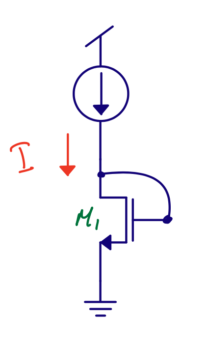
_{Figure 4: Diode connected NMOS biased by a current source, where the current alone sets the operating region}

Use unit size transistors for analog design

\(W/L \approx \in[4, 6, 10]\), but should have space for two contacts

Use parallel transistors for larger W/L

Amplifiers \(\Rightarrow L \approx 1.2 \times L_{min}\)

Current mirrors \(\Rightarrow L \approx 4 \times L_{min}\)

Choose sizes that have been used by foundry for measurement to match SPICE model

What about gm/Id ?

Weak \(\frac{g_m}{I_d} = \frac{1}{nV_T}\)

Strong \(\frac{g_m}{I_d} = \frac{2}{V_{eff}}\)

Characterize the transistors

http://analogicus.com/cnr_atr_sky130nm/mos/CNRATR_NCH_2C1F2.html

More information

Ngspice Manual

Installing tools

Analog Design

Define the problem, what are you trying to solve?
Find a circuit that can solve the problem (papers, books)
Find right transistor sizes. What transistors should be weak inversion, strong inversion, or don’t care?
Check operating region of transistors (.op)
Check key parameters (.dc, .ac, .tran)
Check function. Exercise all inputs. Check all control signals
Check key parameters in all corners. Check mismatch (Monte-Carlo simulation)
Do layout, and check it’s error free. Run design rule checks (DRC). Check layout versus schematic (LVS)
Extract parasitics from layout. Resistance, capacitance, and inductance if necessary.
On extracted parasitic netlist, check key parameters in all corners and mismatch (if possible).
If everything works, then you’re done.

On failure, go back

Demo

https://github.com/analogicus/jnw_spice_sky130A/tree/main

Summary

The one-page version of this chapter:

SPICE has run the same way for fifty-odd years: a netlist in, operating points and waveforms out
The quartet to master: op, dc, ac and tran - everything else is decoration on those four
ngspice speaks the dialect this course uses, and the transistor models come from the PDK, not from the simulator

Would you like to know more?

Nagel’s 1975 thesis, where SPICE comes from, and which still reads well

The ngspice manual, the reference for everything this chapter does