PDF Slides

Table of contents

• Measured Silicon
  • The same physics, read out two ways
• What the silicon does
  • Against a real reference
  • What calibration buys
• The clock in the loop
  • GR07’s output is quantised, and noise is what rescues it
  • When averaging stops helping
  • Two sensors, one event
• One trap
  • GR06 does not drift, it switches
• Summary
• Would you like to know more?

Keywords: Tapeout, Tiny Tapeout, PTAT, Time-domain readout, Temperature chamber, Transfer curve, INL, Calibration, Allan deviation, Quantisation, Dither, Bernoulli statistics, Random telegraph noise

Measured Silicon

The previous chapter set you a project. This one is what happened when two groups finished it.

In the spring of 2025 two groups of three students designed temperature sensors in this course, and both went to a shuttle: Tiny Tapeout project 258, tt_um_jnw_wulffern, on ttsky25a in sky130. The chips came back. This chapter is what they do.

It is here for a specific reason. Everything else in this book is either theory or somebody else’s measurement. This is the one chapter where the circuit was designed by students at your stage, on the tools you are using, and then measured against a temperature chamber - and where the interesting results are not the ones the designers were aiming at.

The same physics, read out two ways

Both sensors are the same idea, and it is the idea the project chapter asks you to build: a current proportional to absolute temperature (PTAT) charging a capacitor, with a comparator watching the ramp. The current comes from the difference between two diode voltages at different current densities, which is the bandgap core of the references chapter,

\[I(T) = \frac{kT}{qR}\ln N\]

and the time to charge $C$ up to a threshold $V_{ref}$ is therefore

\[t = \frac{V_{ref}C}{I(T)} \propto \frac{1}{T}\]

The time falls as the temperature rises, so the rate $1/t$ rises with absolute temperature. Everything measured below is done in the rate domain for that reason: it is the quantity that should be a straight line through the origin.

Both groups built that PTAT core the same way - a pnp of unit area against eight of them, an amplifier forcing the two branch voltages equal, and a resistor setting the current - but not with the same circuit. GR07 puts three RPPO16 in series and mirrors the result straight out, one to one. GR06 uses an RPPO8 and an RPPO4 and then divides its current down through two further mirrors, an NMOS pair ten wide and a PMOS pair ten wide, before it reaches the capacitor. That is roughly a hundredfold division, and it is most of why GR06 runs six times slower on a capacitor a quarter the size.

Both also take their comparator threshold from a resistive divider across the supply rather than from anything absolute: GR07 taps one resistor up from ground in a string of four, so $V_{ref} = V_{DD}/4$; GR06 taps one of three, so $V_{ref} = V_{DD}/3$. Neither threshold is a bandgap voltage. The ratio $V_{ref}/I(T)$ that sets the time therefore carries the supply in it, which is worth remembering before reading any absolute number below as a property of the sensor alone.

Where the two designs really part company is what closes the loop, and that turns out to matter far more than anything in the analogue.

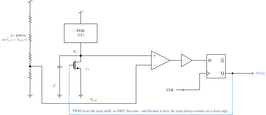
_{Figure 1: GR07, by Reidar Arne Eidsvik Nerheim, Pol Batalle Largo and Tord Olsen Sætermo, drawn from the taped-out netlist. The comparator output is buffered into a D flip-flop clocked by the project clock, and the flip-flop’s output both leaves the chip as PWM and turns on the two NMOS that short the ramp capacitor. The loop closes through the chip, so the sensor free-runs and its period is the observable}

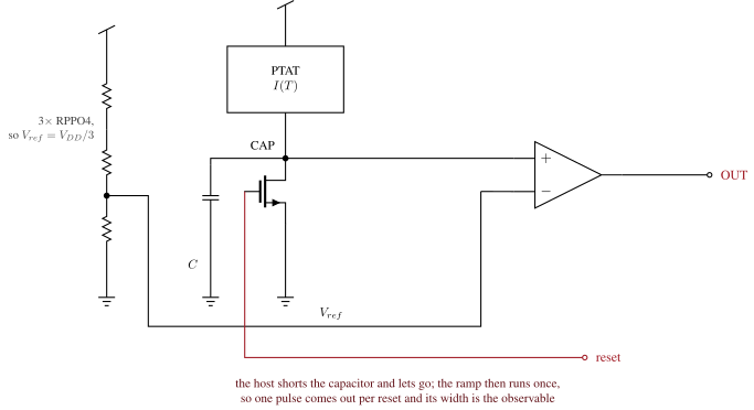
_{Figure 2: GR06, by Gabin Sbaffi, Erik K. Jensen and Renate Klemetsdal. The same front end, and the same NMOS shorting the capacitor - but its gate is a chip input. The host asserts reset, the capacitor discharges, and on release the ramp runs once. One pulse per stimulus, and its width is the observable. Nothing in this circuit is clocked}

At room temperature GR07 free-runs at about 910 kHz - a period near 1.1 µs - so half a second of capture contains half a million periods. GR06 only produces a pulse when the host asks for one, and the host asks about 4.5 thousand times a second, so the same half second contains about 2 300 pulses. GR07 therefore delivers roughly two hundred times more events per measurement, which you would expect to make it the better sensor. Hold that thought.

What the silicon does

Against a real reference

Everything you can do on a bench calibrates a sensor against itself. To find out whether either sensor is right, rather than merely repeatable, you need an outside opinion. A Vötsch temperature chamber stepping from 5 °C to 70 °C in 5 K steps, logging its own probe beside both sensors, supplies one. Each point below is the mean of the last 90 s of a dwell, after both the oven and the die have stopped moving.

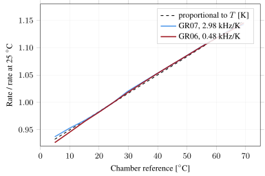
_{Figure 3: Both sensors against the chamber’s own probe, each rate divided by its own value at 25 °C. The dashed line is what a current strictly proportional to absolute temperature would do. Both lie on it: the physics works, and the two designs agree with each other despite a sixfold difference in rate}

Figure 3 is the result the students were designing for, and it is a good one. Two independently designed PTAT cores, built by different people from the same principle, land on the ideal line and on each other. GR07 gives 2.98 kHz/K on 907 kHz; GR06 gives 0.48 kHz/K on 142 kHz. Those are 0.33 %/K and 0.34 %/K - the same fractional slope, which is what “proportional to absolute temperature” means.

Figure 4 is where the two part company. Take the straight line away and both are left with about 1.3 K of something. Now allow one more term - the $T\ln T$ curvature the references chapter warns about, which comes from the temperature dependence of the saturation current in the very diodes that make the PTAT current.

For GR06 that removes almost all of it: 1.33 K peak becomes 0.23 K, and the residual goes flat. GR06’s error is bandgap curvature, and it is the textbook shape at the textbook size.

For GR07 the same term barely helps - 1.61 K becomes 1.04 K - and what is left still wanders. Whatever limits GR07 is not curvature.

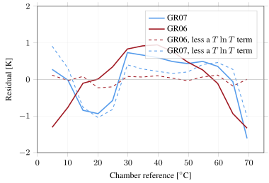
_{Figure 4: What is left of each transfer after the best straight line, and after also allowing a $T\ln T$ term - the bandgap curvature the references chapter warns about. Almost all of GR06’s residual is that curvature. Almost none of GR07’s is}

One caveat on the identification. Over a 65 K span $T\ln T$ and $T^2$ are nearly collinear, and fitting either removes the same amount. The data cannot tell you which functional form it is; what it can tell you is that GR06’s residual is smooth curvature of the size and sign a bandgap predicts, and that GR07’s is not smooth curvature at all.

What calibration buys

The question a product actually asks is not “how linear is it” but “how many oven visits must I pay for”. Every calibration temperature costs money in production, so the interesting curve is error against number of trim points.

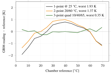
_{Figure 5: GR06’s error after calibrating at one, two and three temperatures. Each extra trim point buys accuracy, ending at ±0.35 K over 5-70 °C. This is what a well-behaved sensor looks like}

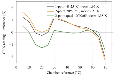
_{Figure 6: The same for GR07, which gets worse going from one point to two}

GR06 does what you would hope: 1.93 K with one point, 1.37 K with two, 0.35 K with three. That is a normal, well-behaved sensor, and ±0.35 K over a 65 K span from three trim points is a respectable number for a first silicon by three students.

GR07 goes 1.96 K, then 2.21 K, then 1.38 K. Getting worse when you give it more information looks like a mistake in the analysis. It is not. A two-point calibration corrects a slope, and GR07’s error is not a slope. Trimming the line just pivots it and drops the residual somewhere else.

To see what GR07’s error actually is, you have to look at what its output is made of.

The clock in the loop

GR07’s output is quantised, and noise is what rescues it

Look again at Figure 1. The comparator trips whenever it trips, but its output reaches the reset transistors through a flip-flop, and a flip-flop can only change at a clock edge. Every GR07 period is therefore a whole number of 64 MHz clock cycles, and nothing in between is representable.

That is not a small quantum. GR07’s period is about seventy clock cycles at room temperature and falls by roughly one cycle for every five kelvin of warming, so one clock cycle is about 4.75 K - three times the whole calibrated error of Figure 6, and larger than the raw uncalibrated error of Figure 4.

A noiseless version of this circuit would be a plain 4.75 K quantiser. Every period would come out the same, and the average of a million of them would tell you no more than one of them did: 4.75 K steps, and nothing in between.

What gets it below that is noise. Jitter on the comparator crossing - from the PTAT current, from the comparator itself, from the supply - is enough to push some periods over the clock edge and not others. Say the crossing sits a fraction $f$ of a cycle past an edge. The output then alternates between $N$ and $N+1$ cycles, and the fraction of periods that come out long is an estimate of $f$. Averaging a million of them reads it to a few millikelvin.

That is dither: noise deliberately relied upon to make a coarse quantiser resolve below its own step. It is the same mechanism that lets a noisy ADC average its way below one LSB, and it is why converters are sometimes given dither on purpose. Here nobody gave it any - the circuit simply happened to have enough.

And a mechanism that depends on noise being big enough has an obvious way to fail.

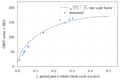
_{Figure 7: GR07’s measured noise against $f$, the fractional part of its period in 64 MHz clock cycles. The dashed curve is $\sqrt{f(1-f)}$ with one scale factor fitted to the data}

The measured noise is not constant: it varies by a factor of eight across the sweep, and it varies with $f$ in a very particular way.

That shape is not a coincidence. If a fraction $f$ of the periods come out long and the rest short, each period is a coin flip with probability $f$ - a Bernoulli trial, whose variance is $f(1-f)$. The spread of a rate estimated from many of them therefore goes as $\sqrt{f(1-f)}$: smallest where the period is nearly a whole number of cycles, largest where it sits half-way between. The dashed curve is that expression with a single scale factor fitted, and it follows the fourteen measurements with a correlation of 0.997.

So GR07’s precision depends on the temperature it happens to be at, through nothing more than the arithmetic of the quantiser. At 10 °C its period is within a hundredth of a whole cycle and its noise is 22 Hz; at 25 °C it sits nearly half-way between and the noise is 186 Hz. Same circuit, same clock, eight times the noise, and it is the fractional part of a division that decides which you get.

This also puts a floor under how well GR07 can ever be trimmed. Calibration fits a smooth function to a transfer; what GR07 delivers is a 4.75 K staircase whose dither statistics change from step to step. The cheapest real fix is not more calibration points but a faster project clock, which shrinks the step in proportion.

GR06, with no clock anywhere in its path, has none of this. Its output is a pulse width in continuous time, and it is limited by something else entirely.

When averaging stops helping

If the resolution comes from averaging, the honest question is how long you can usefully average for. A standard deviation cannot answer it. The Allan deviation can: it asks how repeatable the answer is if you average for $\tau$ seconds, and its slope is the information. Falling means averaging still buys you precision. Rising means drift has taken over and averaging longer makes the answer worse.

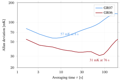
_{Figure 8: Allan deviation of both sensors over fifteen minutes in a quiet room. GR06 is lower at every averaging time. GR07 bottoms out at 57 mK after about eight seconds and then degrades; GR06 keeps improving out past a minute, to 31 mK}

The two-hundred-fold event advantage does not appear anywhere on this plot. GR06 is the better sensor at every averaging time, from the shortest to the longest, and the gap widens.

That is worth sitting with, because within a single half-second capture GR07 really is the more precise of the two: its standard error is 3.3 mK against GR06’s 12.8 mK. But note how little that is. Two hundred times the events should be $\sqrt{200}$, a factor of fifteen, and GR07 only manages four. The missing factor is its own single-event resolution: one GR07 period is worth 2.3 K of scatter against 0.6 K for one GR06 pulse, because 4.75 K of quantiser has to be dithered through. GR07 spends most of its event advantage buying back what the flip-flop took.

The four it keeps then does not survive either. Its Allan deviation at the shortest averaging time is 80 mK - twenty-four times its own statistical error - where GR06’s is 55 mK against 12.8 mK, a factor of four. Both sensors are limited by something other than counting statistics, and GR07 by far the more so. Beyond about ten seconds its curve turns upward, which means something slower than the averaging window is now spoiling the answer and averaging longer makes it worse. GR06, producing two hundred times fewer events, keeps improving.

There is a second result hiding in the same run. Over those fifteen minutes the two sensors’ fluctuations are essentially uncorrelated ($r = 0.11$) despite sitting on the same die, in the same room, sharing a supply. If the wander were the room, both would see it - so it looks like each sensor’s own noise rather than the room.

A quiet room cannot prove that on its own, though: “nothing happened” and “both sensors missed it” look identical from inside. The next section is the experiment that separates them.

Two sensors, one event

Everything so far measures a sensor against a reference. The two sensors on this die can also be measured against each other, which asks a different question: not what is the temperature but did something happen. For that you need something to happen - so, a can of freeze spray, and then a finger held on the package.

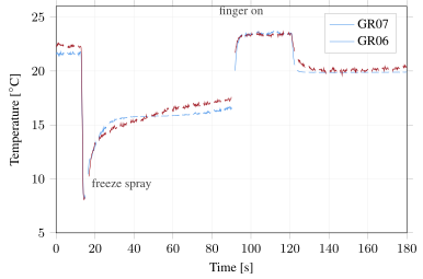
_{Figure 9: A can of freeze spray at 13 s, then a fingertip on the package from 88 s to 122 s, both sensors on one capture. The die falls 13 K in under two seconds, at better than 20 K/s at the steepest. Gaps are dead time between captures, drawn as gaps rather than interpolated}

The two traces do not sit on top of each other - through the long recovery GR06 reads up to about a kelvin above GR07 - but they move together. Every feature appears in both at the same instant, and the correlation of the two temperature series is 0.96 through the spray and recovery and 0.99 while the finger is on.

The offset is not a surprise. Each sensor is calibrated at a single point near 23 °C against the ideal line through the origin, with no offset term to absorb comparator delay or reset time, so at 8 °C both are extrapolating fifteen kelvin beyond their only anchor. What the figure supports is the shape: the timing, the rates, and the fact that both saw the same thing. The absolute depth is the weakest number on the page.

This is the control the previous section needed. Quiet, the two sensors were uncorrelated; given something real to follow, they agree almost perfectly. Both cannot be true of the same physical temperature, and that settles it: the wander in the quiet room was not the room, it was each sensor’s own noise. A real thermal event moves both. Noise moves one.

Which is the argument for putting two of anything on a die. One sensor gives you a number and no way to know whether to believe it. Two give you a way to tell a measurement from an artefact.

Now the same experiment, gently: four breaths on the package.

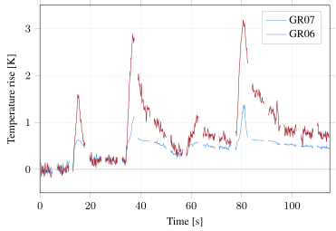
_{Figure 10: Four breaths, both sensors, one capture. Each breath moves both - but GR06 reads about 2.2 times the excursion GR07 does}

Both sensors agree that four things happened, and disagree about how big they were by a factor of 2.2. The obvious reading is that the two circuits have different gains. They do not: over the 15 K of Figure 9 they agree to within a few per cent, and a real gain error would show up more strongly over a wider excursion, not vanish.

So something compresses GR07’s response to small, fast signals without touching its response to large slow ones. A one-kelvin breath is about a fifth of GR07’s 4.75 K quantiser step, so the quantiser is the obvious suspect - but the chamber sweep of Figure 7 shows its dither behaving the way ideal dither should, which would give a linear response at any excursion. The two observations are not yet reconciled, and nothing else measured here settles it.

What can be said without hand-waving is the practical part: for small, fast signals the two sensors disagree by a factor of about two, and GR06 is the one that agrees with the larger excursion. Trust it. Establishing why would need a controlled small-step experiment with GR07 parked at several known values of $f$ - which is a good project, and is not in this data set.

One trap

GR06 does not drift, it switches

GR06 is the better-behaved sensor everywhere above, so it is worth asking what actually limits it. Hold the chamber still and look at a minute of GR06 with the slow dwell drift removed.

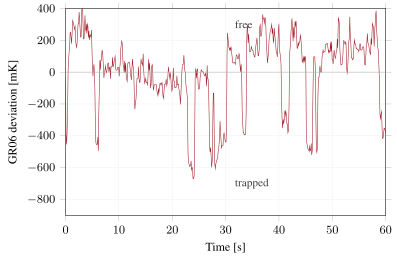
_{Figure 11: Sixty seconds of GR06 at a fixed chamber temperature, with the slow dwell drift removed. The reading sits flat, drops about six tenths of a kelvin to a second level, stays there a second or two, and comes back}

Thermal noise would give a fuzzy band around zero. This gives two levels. That is random telegraph noise - a single charge trap in the silicon capturing and emitting one carrier - and it is the same mechanism the noise chapter introduces as the microscopic origin of flicker noise, here big enough to see one trap at a time.

The step is about 0.6 K from 5 °C to 55 °C - it drifts from 0.7 K to 0.4 K across that span, but it does not scale with anything - which says it is one trap rather than a population. The time it stays trapped is thermally activated and follows an Arrhenius law, which is what identifies it as a trap rather than as something in the instrument.

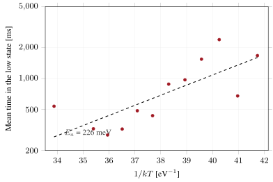
_{Figure 12: The trap’s mean lifetime in the low state against inverse thermal energy, one point per chamber dwell. A straight line here is an Arrhenius law; the slope is an activation energy of 226 meV. Above about 55 °C the two levels merge into the noise and the fit stops meaning anything, so those dwells are left out}

So GR06’s real single-reading accuracy is not its ±0.35 K three-point calibration - that is a ninety-second mean. A single reading can be six tenths of a kelvin off whenever the trap happens to be occupied. Unlike GR07’s quantiser this is cheap to fix: a median over a second or two steps straight over it.

Summary

Two sensors from this course, on the same die, from the same principle.

• Both PTAT cores work. The rates follow absolute temperature to within the residual of Figure 3, and the two designs - different resistors, and a hundredfold current division in one of them - agree with each other to a per cent in fractional slope.
• GR06, with three calibration points, is accurate to ±0.35 K over 5-70 °C. What is left after a straight line is bandgap curvature: a $T\ln T$ term takes 1.33 K down to 0.23 K. Its limit for a single reading is not linearity at all but one charge trap worth about 0.6 K, which a short median removes.
• GR07 has four times GR06’s statistical precision within a capture and is the worse sensor at every averaging time - its readings scatter twenty-four times more than its own statistics predict. Its output is quantised to whole clock cycles, 4.75 K each, and only noise dithering the crossing lets averaging resolve below that. How precise it is then depends on where it sits in that step: the noise follows $\sqrt{f(1-f)}$ to a correlation of 0.997, an eightfold range across the sweep, decided by the fractional part of a division.
• Calibration cannot absorb a staircase. A faster clock shrinks it.
• The two sensors’ noise is uncorrelated on one die. Two sensors tell you when something is real; one tells you a number.

If you take one thing from this chapter into your own project: both groups’ analogue cores did what they were designed to do. Every awkward result came from the boundary - a flip-flop, a clock frequency, a choice of what to observe. That is where to spend your attention.

Would you like to know more?

The measurement setup, the full analysis and every figure’s underlying data, in far more detail than fits here ¹

The Tiny Tapeout shuttle that carried it, and how to put your own design on one ²

Where the PTAT core comes from, and why its curvature is not what limits these parts ³

Quantisation, dither and why a coarse converter with noise on its input beats a coarse converter without ⁴

Random telegraph noise as the microscopic origin of flicker noise ⁵

1. Carsten Wulff, JNW-TEMP: two temperature sensors, measured 2026 https://analogicus.com/jnw-tt-2025/presentation.html ↩

2. Matt Venn and the Tiny Tapeout contributors, Tiny Tapeout https://tinytapeout.com ↩

3. B. Razavi, The Design of a Low-Voltage Bandgap Reference [The Analog Mind] 2021 https://doi.org/10.1109/MSSC.2021.3088963 ↩

4. Richard Schreier and Garbor C. Temes, Understanding Delta-Sigma Data Converters 2005 ↩

5. M. J. Kirton and M. J. Uren, Noise in solid-state microstructures: A new perspective on individual defects, interface states and low-frequency (1/f) noise 1989 https://doi.org/10.1080/00018738900101122 ↩