analysis
- Waveform interaction
- Keyboard shortcuts
- Mouse controls
- Wave browser
- Digital signals
- Analysis tools
- Session management
Waveform interaction
| Action | Effect |
|---|---|
| Mouse wheel | Zoom in/out |
| Middle click + drag | Pan |
| Right click | Context menu with analysis tools |
| Ctrl+A | Auto-fit all waveforms |
| Ctrl+Mouse wheel | Zoom X-axis only |
Keyboard shortcuts
File
| Key | Action |
|---|---|
| Ctrl+O | Open file |
| Ctrl+S | Save session |
| Ctrl+P | Export to PDF/PNG/SVG |
| Ctrl+Q | Quit |
Edit
| Key | Action |
|---|---|
| Ctrl+N | New plot tab |
| Ctrl+W | Close current tab |
| Ctrl+L | Set axis labels |
| Ctrl+T | Add annotation |
| R | Reload all waveforms |
| F | Auto scale (fit all) |
| Z | Zoom in |
| Shift+Z | Zoom out (Ctrl+Z also works) |
| D | Toggle focused wave between analog and digital pane |
Cursors
| Key | Action |
|---|---|
| A | Set cursor A at mouse position |
| B | Set cursor B at mouse position |
| Escape | Clear cursors |
When two cursors are placed the readout panel shows ΔX, per-signal ΔY, slope, and derivative values at both cursor positions.
View
| Key | Action |
|---|---|
| L | Toggle legend |
| Ctrl+Up | Increase line width |
| Ctrl+Down | Decrease line width |
| Ctrl+= | Increase font size |
| Ctrl+- | Decrease font size |
Mouse controls
| Action | Effect |
|---|---|
| Scroll | Zoom x-axis |
| Shift+Scroll | Zoom y-axis |
| Right-drag | Rubber-band zoom (2D) |
| Shift+Right-drag | Rubber-band zoom (X only) |
| Ctrl+Right-drag | Rubber-band zoom (Y only) |
| Left-drag | Pan |
| Click cursor line | Drag to reposition |
Wave browser
- Double-click a wave to add it to the plot
- Right-click a wave to open the context menu:
- Plot / Remove from plot
- Change plot style (Lines, Markers, Lines+Markers, Steps)
- FFT / PSD (spectral density in dB)
- Histogram (distribution with Gaussian fit, mean/sigma)
- Differentiate (numerical dy/dx)
- X vs Y (parametric plot with regex signal picker)
- Constellation (IQ scatter with symbol timing and carrier-offset correction)
- Signal names with dotted hierarchy (e.g.
v(xdut.x1.out)) are shown as a collapsible tree organized by instance path - Use the Flat checkbox to switch to a flat list view
- Use the regex filter to search for signals
- Plotted waves are colored in the browser to match their plot line
Digital signals
There’s a dedicated digital pane that appears below the analog plot whenever any wave is shown as digital. Traces are rendered gtkwave/surfer-style: 0/1 step lines for single-bit signals, hexagonal bus outlines with value labels for vectors. The digital pane shares the analog x-axis so panning and zooming stay in sync.
VCD files
.vcd files (Verilog Value Change Dump) are loaded directly. Every
signal is parsed, hierarchy is preserved (the . separator becomes tree
levels in the wave browser), and signals are tagged as bit or vector
based on their declared width. Real-valued VCD signals are loaded as
ordinary analog waves.
cicwave dump.vcd
Showing analog waves as digital
Any waveform — including signals from .raw files — can be displayed on
the digital pane. A 0/1 trace is synthesized from the analog data using a
(max + min) / 2 threshold with small hysteresis to suppress noise
around the cross point. Useful for quickly visualising clock or
oscillator outputs from a transient simulation.
Toggle digital mode for the focused wave with the D key, or via the wave browser’s right-click menu (Show as digital). For vector signals the menu also offers a Digital format sub-menu (Hex / Dec / Bin).
Analysis tools
Right-click a trace in the wave tree for the analysis menu:
- Cursors: A/B markers measure time / voltage differences
- FFT / PSD: Hanning-windowed spectrum (peak-normalised dB)
- ADC PSD (SNDR, SFDR, harmonics)…: ADC characterisation
- SNR / SNDR / ENOB…: numeric metrics with the same backend
- Histogram: distribution + Gaussian fit
- Differentiate (dy/dx): numerical derivative
- Linear fit…, Difference (this − other)…, X vs Y…
- Constellation (IQ)…: I/Q scatter of a complex
iqcolumn, or of anIcolumn paired with itsQ(picked for you when the names match). Set the sample rate (prefilled from SigMF /.npzsidecar /.iqvsa/ audio file metadata or the time axis), a symbol rate to take one point per symbol (fractional samples per symbol are fine), a timing offset in samples to land on the symbol centre, and a frequency offset (Hz) and phase to derotate a radio’s carrier offset. For SigMF recordings with annotations, pick an annotated range (the first complete one is preselected) so the idle gaps stay out. Any labelled range works, so a recording whose metadata also annotates the sections of each packet ("core:label": "header","payload", …) shows each section’s constellation on its own; cicwave needs no knowledge of the protocol. A window start/stop in µs narrows the selection further; low-IF captures prefill the channel offset and the spectrum-inverted flag. Optionally draws the trajectory behind the symbols; the analysis itself iscicwave.analysis.constellation() - 2’s complement decode submenu: 8 / 10 / 12 / 16-bit signed
- Math expressions: create derived signals
- Digital analysis: bus values and timing
- Export data: save currently visible waveforms
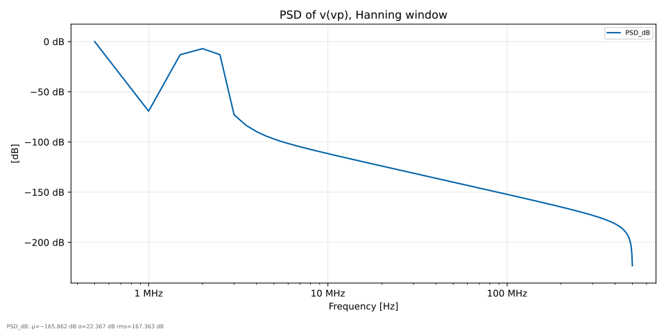
FFT / PSD example
The right-click FFT / PSD action isn’t scriptable from a session file
yet — it’s an interactive GUI action, not a declarative wave type. The
plot below is still a real cicwave PSD, though:
tests/docs/gen_testdata.py calls the same
psd_rfft
backend the menu action uses, on the v(vp) tone from the single
wave example, and plots the resulting
spectrum like any other CSV.
(session_spectrum.cicwave.yaml)
cicwave --session session_spectrum.cicwave.yaml --export wave_spectrum.svg
ADC PSD dialog
Tailored for ADC bench data and behavioural simulations, inspired by
oct_dofft.m / dofftsd.m:
| Field | Meaning |
|---|---|
Sample rate F_s |
Empty → infer from the time axis |
Fundamental F₀ |
Empty / 0 → auto (strongest non-DC bin, with DC and Nyquist guard bands) |
Oversampling OSR |
>1 integrates noise only over the in-band slice (1 … N_fft / OSR), σΔ-style |
Max harmonic order |
Default 5 (H2…H5 typical for ADC reports) |
Harmonic lobe ±bins |
Half-width for the harmonic masks. Hann main lobe is 3 bins; ±3 (7 bins) is a safe default for non-coherent captures |
Fundamental lobe ±bins |
Separate width for the fundamental — use a wider window when jitter or drift smears the tone more than the harmonics |
Full-scale amplitude A_FS |
Peak FS sine amplitude (same units as y). Empty → spectrum is dBc; set → dBFS plot + Signal level = … dBFS line |
Exclude harmonics from SNR… |
Splits SNR vs SNDR (default on); off matches σΔ “in-band noise only” |
Logarithmic frequency axis |
Default on; dialog and markers stay aligned in either mode |
Reported metrics (per call, also shown as a banner on the main wave tab):
SNR,SNDR,ENOB(dynamic_parametersbackend)SFDR— IEEE definition: ratio of fundamental lobe to the largest spur, harmonics included (always in dBc)Hntable — for each harmonic up to Max: integratedlobe power(dBc) andpeakbin (dBc)- Fundamental + harmonics drawn as vertical markers, with diamond glyphs at the spectrum peak nearest each tone
All dialog fields are persisted between invocations via QSettings
(cicwave/cicwave/{snr_dialog,adc_psd_dialog}/…), so running ADC PSD on
the next signal reuses the same F_s, A_FS, lobe widths and so on.
See Pivot for running
dynamic_parameters/rms headlessly via --pivot + --export.
Session management
- File → Save Session: Save current plot configuration
- File → Load Session: Restore previous analysis
- Sessions store: visible signals, zoom levels, cursor positions, analysis setup
See Sessions for the full session file format.