Lecture 6 - Oversampling and Sigma-Delta ADCs
If you find an error in what I’ve made, then fork, fix lectures/l06_adc.md, commit, push and create a pull request. That way, we use the global brain power most efficiently, and avoid multiple humans spending time on discovering the same error.
ADC state-of-the-art
The performance of an analog-to-digital converter is determined by the effective number of bits (ENOB), the power consumption, and the maximum bandwidth.
The effective number of bits contains information on the linearity of the ADC. The power consumption shows how efficient the ADC is. The maximum bandwidth limits what signals we can sample and reconstruct in digital domain.
Many years ago, Robert Walden did a study of ADCs, one of the plot’s is shown below.
1999, R. Walden: Analog-to-digital converter survey and analysis
There are obvious trends, the faster an ADC is, the less precise the ADC is ( lower SNDR). There are also fundamental limits, Heisenberg tells us that a 20-bit 10 GS/s ADC is impossible, according to Walden.
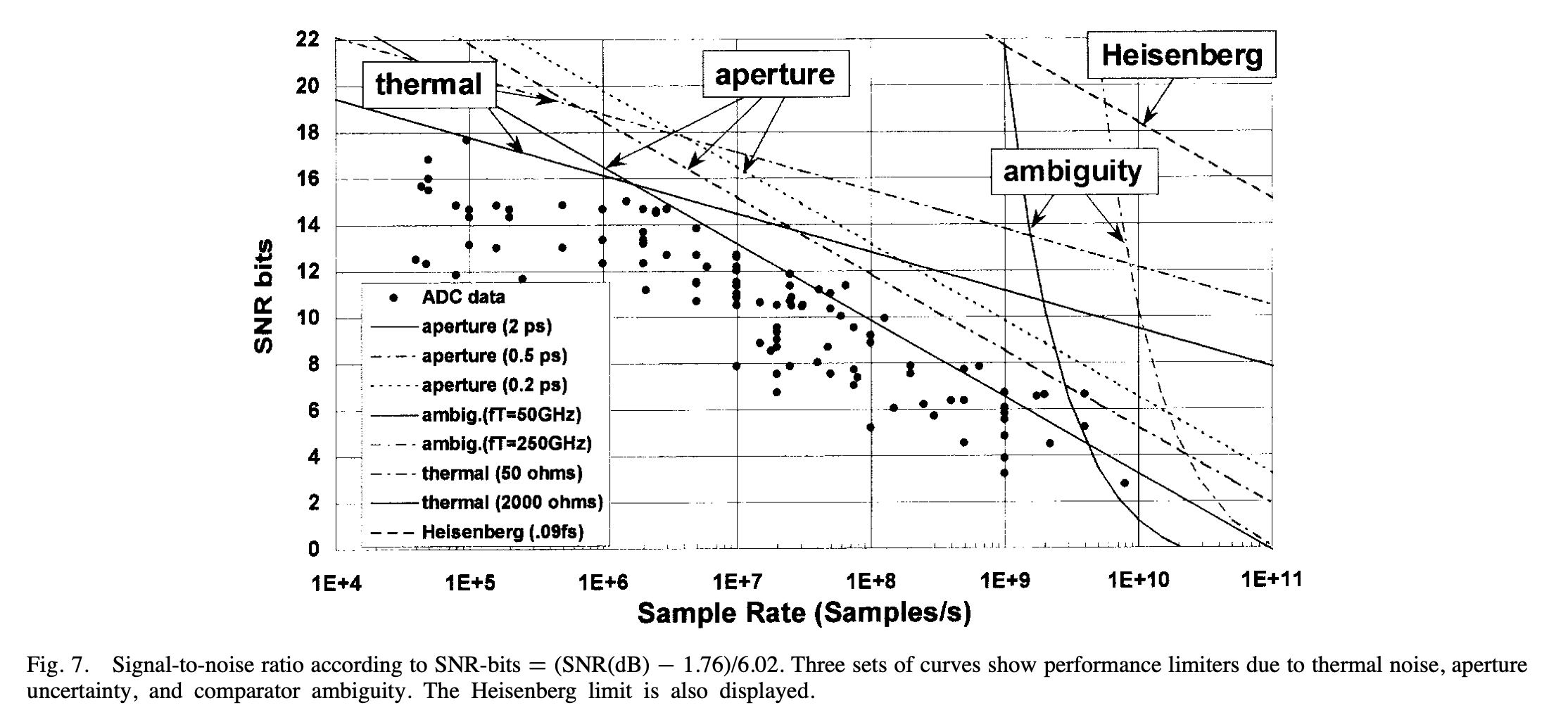
I would take those fundamental limits with a grain of salt. The uncertainty principle states that the precision we can determine position and the momentum of a particle is \(\sigma_x \sigma_p \ge \frac{\hbar}{2}\) In the paper, however, Walden quickly states that \(\Delta E \Delta t > \frac{h}{2 \pi}\) where $\Delta E$ is the difference in energy, and $\Delta t$ is the difference in time. Whether that is a valid reformulation of the uncertainty principle, I’m not sure. Also, the plot assumes 50 Ohm and 1 V full-scale. As a result, the “Heisenberg” line that appears to be unbreakable certainly is breakable. Just change the voltage to 100 V, and the number of bits can be much higher. Always check the assumptions.
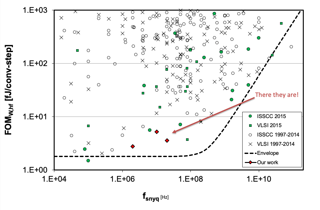
A more recent survey of ADCs comes from Boris Murmann. He still maintains a list of the best ADCs from ISSCC and VLSI Symposium.
B. Murmann, ADC Performance Survey 1997-2022 (ISSCC & VLSI Symposium)
A common figure of merit for low-to-medium resolution ADCs is the Walden figure of merit, defined as
\[FOM_W = \frac{P}{2^B f_s}\]Below 10 fJ/conv.step is good.
Below 1 fJ/conv.step is extreme.
In the plot below you can see the ISSCC and VLSI ADCs.

People from NTNU have made some of the worlds best ADCs
If you ever want to make an ADC, and you want to publish the measurements, then you must be better than most. A good algorithm for state-of-the-art ADC design is to first pick a sample rate with low number of data (blank spaces in the plot above), then read the papers in the vicinity of the blank space to understand the application, then set a target FOM which is best in world, then try and find a ADC architecture that can achieve that FOM.
That’s pretty much the algorithm I, and others, have followed to make state-of-the-art ADCs. A few of the NTNU ADCs are:
A Compiled 9-bit 20-MS/s 3.5-fJ/conv.step SAR ADC in 28-nm FDSOI for Bluetooth Low Energy Receivers
A 68 dB SNDR Compiled Noise-Shaping SAR ADC With On-Chip CDAC Calibration
For high-resolution ADCs, it’s more common to use the Schreier figure of merit, which can also be found in
B. Murmann, ADC Performance Survey 1997-2022 (ISSCC & VLSI Symposium)
The Walden figure of merit assumes that thermal noise does not constrain the power consumption of the ADC, which is usually true for low-to-medium resolution ADCs. To keep the Walden FOM you can double the power for a one-bit increase in ENOB. If the ADC is limited by thermal noise, however, then you must quadruple the capacitance (reduce $kT/C$ noise power) for each 1-bit ENOB increase. Accordingly, the power must also go up four times.
For higher resolution ADC the power consumption is set by thermal noise, and the Schreier FOM allows for a 4x power consumption increase for each added bit.
\[FOM_S = SNDR + 10\log\left(\frac{f_s/2}{P}\right)\]Above 180 dB is extreme

Quantization
Sampling turns continuous time into discrete time. Quantization turns continuous value into discrete value. Any complete ADC is always a combination of sampling and quantization.
In our mathematical drawings of quantization we often define $y[n]$ as the output, the quantized signal, and $x[n]$ as the discrete time, continuous value input, and we add some “noise”, or “quantization noise” $e[n]$, where $x[n] = y[n] - e[n]$.

Maybe you’ve even heard the phrase “Quantization noise is white” or “Quantization noise is a random Gaussian process”?
I’m here to tell you that you’ve been lied to. Quantization noise is not white, nor is it a Gaussian process. Those that have lied to you may say “yes, sure, but for high number of bits it can be considered white noise”. I would say that’s similar to saying “when you look at the earth from the moon, the surface looks pretty smooth without bumps, so let’s say the earth is smooth with no mountains”.
I would claim that it’s an unnecessary simplification. It’s obvious to most that the earth would appear smooth from really far away, but they would not surprised by Mount Everest, since they know it’s not smooth.
An Alien that has been told that the earth is smooth, would be surprised to see Mount Everest.
But if Quantization noise is not white, what is it?
The figure below shows the input signal x and the quantized signal y.

To see the quantization noise, first take a look at the sample and held version of $x$ in green in the figure below. The difference between the green ($x$ at time n) and the red ($y$) would be our quantization noise $e$.
The quantization noise is contained between $+\frac{1}{2}$ Least Significant Bit (LSB) and $-\frac{1}{2}$ LSB.
This noise does not look random to me, but I can’t see what it is, and I’m pretty sure I would not be able to work it out either.

Luckily, there are people in this world that love mathematics, and that can delve into the details and figure out what $e[n]$ is. A guy called Blachman wrote a paper back in 1985 on quantization noise.
See The intermodulation and distortion due to quantization of sinusoids for details
In short, quantization noise is defined as
\[e_n(t) = \sum_{p=1}^\infty{A_p\sin{p\omega t}}\]where p is the harmonic index, and
\[A_p = \begin{cases} \delta_{p1}A + \sum_{m = 1}^\infty{\frac{2}{m\pi}J_p(2m\pi A)} &, p = \text{ odd} \\ 0 &, p = \text{ even} \end{cases}\] \[\delta_{p1} \begin{cases} 1 &, p=1 \\ 0 &, p \neq 1 \end{cases}\]and \(J_p(x)\) is a Bessel function of the first kind, A is the amplitude of the input signal.
If we approximate the amplitude of the input signal as
\[A = \frac{2^n - 1}{2} \approx 2^{n-1}\]where n is the number of bits, we can rewrite as
\[e_n(t) = \sum_{p=1}^\infty{A_p\sin{p\omega t}}\] \[A_p = \delta_{p1}2^{n-1} + \sum_{m=1}^\infty{\frac{2}{m\pi}J_p(2m\pi 2^{n-1})}, p=odd\]Obvious, right?
I must admit, it’s not obvious to me. But I do understand the implications. The quantization noise is an infinite sum of input signal odd harmonics, where the amplitude of the harmonics is determined by a sum of a Bessel function.
A Bessel function of the first kind looks like this

So I would expect the amplitude to show signs of oscillatory behavior for the harmonics. That’s the important thing to remember. The quantization noise is odd harmonics of the input signal
The mean value is zero
\[\overline{e_n(t)} = 0\]and variance (mean square, since mean is zero), or noise power, can be approximated as
\[\overline{e_n(t)^2} = \frac{\Delta^2}{12}\]Signal to Quantization noise ratio
Assume we wanted to figure out the resolution, or effective number of bits for an ADC limited by quantization noise. A power ratio, like signal-to-quantization noise ratio (SQNR) is one way to represent resolution.
Take the signal power, and divide by the noise power
\[SQNR = 10 \log\left(\frac{A^2/2}{\Delta^2/12}\right) = 10 \log\left(\frac{6 A^2}{\Delta^2}\right)\] \[\Delta = \frac{2A}{2^B}\] \[SQNR = 10 \log\left(\frac{6 A^2}{4 A^2/2^B}\right) = 20 B \log 2 + 10 \log 6/4\] \[SQNR \approx 6.02 B + 1.76\]You may have seen the last equation before, now you know where it comes from.
Understanding quantization
Below I’ve tried to visualize the quantization process q.py.
The left most plot is a sinusoid signal and random Gaussian noise. The signal is not a continuous time signal, since that’s not possible on a digital computer, but it’s an approximation.
The plots are FFTs of a sinusoidal signal combined with noise. These are complex FFTs, so they show both negative and positive frequencies. The x-axis is the FFT bin (not the frequency). Notice that there are two spikes, which should not be surprising, since a sinusoidal signal is a combination of two frequencies.
\[sin(x) = \frac{e^{ix} - e^{-ix}}{2i}\]The second plot from the left is after sampling, notice that the noise level increases. The increase in the noise level should be due to noise folding, and reduced number of points in the FFT, but I have not confirmed (maybe you could confirm?).
The right plot is after quantization, where I’ve used the function below.
def adc(x,bits):
    levels = 2**bits
    y = np.round(x*levels)/levels
    return y
I really need you to internalize a few things from the right most plot. Really think through what I’m about to say.
Can you see how the noise (what is not the two spikes) is not white? White noise would be flat in the frequency domain, but the noise is not flat.

If you run the python script you can zoom in and check the highest spikes. The fundamental is at 127, so odd harmonics would be 381, 635, 889, and from the function of the quantization noise we would expect those to be the highest harmonics (at least when we look at the Bessel function), however, we can see that it’s close, but that bin 396 is the highest. Is the math’s wrong?
No, the math is correct. Never bet against mathematics. If you change the python script to reduce the frequency, fdivide=2**9, and increase number of points, N=2**16, as in the plot below, you’ll see it’s the 11’th harmonic that is highest.

All the other spikes are the odd harmonics above the sample rate that fold. The infinite sum of harmonics will fold, some in-phase, some out of phase, depending on the sign of the Bessel function.
From the function for the amplitude of the quantization noise for harmonic indices higher than $p=1$
\[A_p = \sum_{m=1}^\infty{\frac{2}{m\pi}J_p(2m\pi \bf{2^{n-1}})}, p=odd\]we can see that the input to the Bessel function increases faster for a higher number of bits $n$. As such, from the Bessel function figure above, I would expect that the sum of the Bessel function is a lower value. Accordingly, the quantization noise reduces at higher number of bits.
A consequence is that the quantization noise becomes more and more uniform, as can be seen from the plot of a 10-bit quantizer below. That’s why people say “Quantization noise is white”, because for a high number of bits, it looks white in the FFT.

Why you should care about quantization noise
So why should you care whether the quantization noise looks white, or actually is white? A class of ADCs called oversampling and sigma-delta modulators rely on the assumption that quantization noise is white. In other words, the cross-correlation between noise components at different time points is zero. As such the noise power sums as a sum of variance, and we can increase the signal-to-noise ratio.
We know that assumption to be wrong though, quantization noise is not white. For noise components at harmonic frequencies the cross-correlation will be high. As such, when we design oversampling or sigma-delta based ADC we will include some form of dithering (making quantization noise whiter). For example, before the actual quantizer we inject noise, or we make sure that the thermal noise is high enough to dither the quantizer.
Everybody that thinks that quantization noise is white will design non-functioning (or sub-optimal) oversampling and sigma-delta ADCs. That’s why you should care about the details around quantization noise.
Oversampling
Assume a signal $x[n] = a[n] + b[n]$ where $a$ is a sampled sinusoid and $b$ is a random process where cross-correlation is zero for any time except for $n=0$. Assume that we sum two (or more) equally spaced signal components, for example
\[y = x[n] + x[n+1]\]What would the signal to noise ratio be for $y$?
Noise power
Our mathematician friends have looked at this, and as long the noise signal $b$ is random then the noise power for the oversampled signal $b_{osr} = b[n] + b[n+1]$ will be
\[\overline{b_{osr}^2} = OSR \times \overline{b^2}\]where OSR is the oversampling ratio. If we sum two time points the $OSR=2$, if we sum 4 time points the $OSR=4$ and so on.
For fun, let’s go through the mathematics
Define $b_1 = b[n]$ and $b_2 = b[n+1]$ and compute the noise power
\[\overline{(b_1 + b_2)^2} = \overline{b_1^2 + 2b_1b_2 + b_2^2}\]Let’s replace the mean with the actual function
\[\frac{1}{N}\sum_{n=0}^N{\left(b_1^2 + 2b_1b_2 + b_2^2\right)}\]which can be split up into
\[\frac{1}{N}\sum_{n=0}^N{b_1^2} + \frac{1}{N}\sum_{n=0}^N{2b_1b_2} + \frac{1}{N}\sum_{n=0}^N{b_2^2}\]we’ve defined the cross-correlation to be zero, as such
\[\overline{(b_1 + b_2)^2} = \frac{1}{N}\sum_{n=0}^N{b_1^2} + \frac{1}{N}\sum_{n=0}^N{b_2^2} = \overline{b_1^2} + \overline{b_2^2}\]but the noise power of each of the $b$’s must be the same as $b$, so
\[\overline{(b_1 + b_2)^2} = 2\overline{b^2}\]Signal power
For the signal $a$ we need to calculate the increase in signal power as OSR increases.
I like to think about it like this. $a$ is low frequency, as such, samples $n$ and $n+1$ is pretty much the same value. If the sinusoid has an amplitude of 1, then the amplitude would be 2 if we sum two samples. As such, the amplitude must increase with the OSR.
The signal power of a sinusoid is $A^2/2$, accordingly, the signal power of an oversampled signal must be $(OSR \times A)^2/2$.
Signal to Noise Ratio
Take the signal power to the noise power
\[\frac{(OSR \times A)^2/2}{OSR \times \overline{b^2}} = OSR \times \frac{A^2/2}{\overline{b^2}}\]We can see that the signal to noise ratio increases with increased oversampling ratio, as long as the cross-correlation of the noise is zero
Signal to Quantization Noise Ratio
The in-band quantization noise for a oversampling ratio (OSR)
\[\overline{e_n(t)^2} =\frac{\Delta^2}{12 OSR}\]And the improvement in SQNR can be calculated as
\[SQNR = 10 \log\left(\frac{6 A^2}{\Delta^2/OSR}\right) = 10 \log\left(\frac{6 A^2}{\Delta^2}\right) + 10 \log(OSR)\] \[SQNR \approx 6.02B + 1.76 + 10 \log(OSR)\]For an OSR of 2 and 4 the SQNR improves by
\[10 \log(2) \approx 3 dB\]and for OSR=4
\[10 \log(4) \approx 6 dB\]which is roughly equivalent to a 0.5-bit per doubling of OSR
Python oversample
There are probably more elegant (and faster) ways of implementing oversampling in python, but I like to write the dumbest code I can, simply because dumb code is easy to understand.
Below you can see an example of oversampling. The oversample function takes in a
vector and the OSR. For each index it sums OSR future values.
def oversample(x,OSR):
    N = len(x)
    y = np.zeros(N)

    for n in range(0,N):
        for k in range(0,OSR):
            m = n+k
            if (m < N):
                y[n] += x[m]
    return y
Below we can see the plot for OSR=2, the right most plot is the oversampled version.
The noise has all frequencies, and it’s the high frequency components that start to cancel each other. An average filter (sometimes called a sinc filter due to the shape in the frequency domain) will have zeros at $\pm fs/2$ where the noise power tends towards zero.

The low frequency components will add, and we can notice how the noise power increases close to the zero frequency (middle of the x-axis).
For an OSR of 4 we can notice how the noise floor has 4 zero’s.

The code for the plots is osr.py. I would encourage you to play a bit with the code, and make sure you understand oversampling.
Noise Shaping
Look at the OSR=4 plot above. The OSR=4 does decrease the noise compared to the discrete time discrete value plot, however, the noise level of the discrete time continuous value is much lower.
What if we could do something, add some circuitry, before the quantization such that the quantization noise was reduced?
That’s what noise shaping is all about. Adding circuits such that we can “shape” the quantization noise. We can’t make the quantization noise disappear, or indeed reduce the total noise power of the quantization noise, but we can reduce the quantization noise power for a certain frequency band.
But what circuitry can we add?
The magic of feedback
A generalized feedback system is shown below, it could be a regulator, a unity-gain buffer, or something else.
The output $V_o$ is subtracted from the input $V_i$, and the error $V_x$ is shaped by a filter $H(s)$.
If we make $H(s)$ infinite, then $V_o = V_i$. If you’ve never seen such a circuit, you might ask “Why would we do this? Could we not just use $V_i$ directly?”. There are many reasons for using a circuit like this, let me explain one instance.
Imagine we have a VDD of 1.8 V, and we want to make a 0.9 V voltage for a CPU. The CPU can consume up to 10 mA. One way to make a divide by two circuit is with two equal resistors connected between VDD and ground. We don’t want the resistive divider to consume a large current, so let’s choose 1 MOhm resistors. The current in the resistor divider would then be about 1 $\mu$A. We can’t connect the CPU directly to the resistor divider, the CPU can draw 10 mA. As such, we need a copy of the voltage at the mid-point of the resistor divider that can drive 10 mA.
Do you see now why a circuit like the one below is useful? If not, you should really come talk to me so I can help you understand.

Sigma-delta principle
Let’s modify the feedback circuit into the one below. I’ve added an ADC and a DAC to the feedback loop, and the $D_o$ is now the output we’re interested in. The equation for the loop would be
\[D_o = adc\left[H(s)\left(dac(D_o) - V_i\right)\right]\]But how can we now calculate the transfer function $\frac{D_o}{V_i}$? Both $adc$ and $dac$ could be non-linear functions, so we can’t disentangle the equation. Let’s make assumptions.

The DAC assumption
Assumption 1: the $dac$ is linear, such that $V_o = dac(D_o) = A D_o + B$, where $A$ and $B$ are scalar values.
The DAC must be linear, otherwise our noise-shaping ADC will not work.
One way to force linearity is to use a 1-bit DAC, which has only two points, so should be linear. For example \(V_o = A \times D_o\), where $D_o \in (0,1)$. Even a 1-bit DAC could be non-linear if $A$ is time-variant, so $V_o[n] = A(t)\times D_o[n]$, this could happen if the reference voltage for the DAC changed with time.
I’ve made a couple noise shaping ADCs, and in the first one I made I screwed up the DAC. It turned out that the DAC current had a signal dependent component which lead to a non-linear behavior.
The ADC assumption
Assumption 2: the $adc$ can be modeled as a linear function $D_o = adc(x) = x + e$, where e is white noise source
We’ve talked about this, the $e$ is not white, especially for low-bit ADCs, so we usually have to add noise. Sometimes it’s sufficient with thermal noise, but often it’s necessary to add a random, or pseudo-random noise source at the input of the ADC.
The modified equation
With the assumptions we can change the equation into
\[D_o = adc\left[H(s)\left(V_i - dac(D_o)\right)\right] = H(s)\left( V_i - A D_o\right) + e\]In noise-shaping texts it’s common to write the above equation as
\[y = H(s)(u - y) + e\]or in the sample domain
\[y[n] = e[n] + h*(u[n] - y[n])\]which could be drawn in a signal flow graph as below.

in the Z-domain the equation would turn into
\[Y(z) = E(z) + H(z)\left[U(z) - Y(z)\right]\]The whole point of this exercise was to somehow shape the quantization noise, and we’re almost at the point, but to show how it works we need to look at the transfer function for the signal $U$ and for the noise $E$.
Signal transfer function
Assume U and E are uncorrelated, and E is zero
\[Y = HU - HY\] \[STF = \frac{Y}{U} = \frac{H}{1 + H} = \frac{1}{1 + \frac{1}{H}}\]Imagine what will happen if H is infinite. Then the signal transfer function (STF) is 1, and the output $Y$ is equal to our input $U$. That’s exactly what we wanted from the feedback circuit.
Noise transfer function
Assume U is zero
\[Y = E + HY \rightarrow NTF = \frac{1}{1 + H}\]Imagine again what happens when H is infinite. In this case the noise-transfer function becomes zero. In other words, there is no added noise.
Combined transfer function
In the combined transfer function below, if we make $H(z)$ infinite, then $Y = U$ and there is no added quantization noise. I don’t know how to make $H(z)$ infinite everywhere, so we have to choose at what frequencies it’s “infinite”.
\[Y(z) = STF(z) U(z) + NTF(z) E(z)\]There are a large set of different $H(z)$ and I’m sure engineers will invent new ones. We usually classify the filters based on the number of zeros in the NTF, for example, first-order (one zero), second order (two zeros) etc. There are books written about sigma-delta modulators, and I would encourage you to read those to get a deeper understanding. I would start with Delta-Sigma Data Converters: Theory, Design, and Simulation.
First-Order Noise-Shaping
We want an infinite $H(z)$. One way to get an infinite function is an accumulator, for example
\[y[n+1] = x[n] + y[n]\]or in the Z-domain
\[zY = X + Y \rightarrow Y(z-1) = X\]which has the transfer function
\[H(z) = \frac{1}{z-1}\]The signal transfer function is
\[STF = \frac{1/(z-1)}{1 + 1/(z-1)} = \frac{1}{z} = z^{-1}\]and the noise transfer function
\[NFT = \frac{1}{1 + 1/(z-1)} = \frac{z-1}{z} = 1 - z^{-1}\]In order calculate the Signal to Quantization Noise Ratio we need to have an expression for how the NTF above filters the quantization noise.
In the book they replace the $z$ with the continuous time variable
\[z = e^{sT} \overset{s=j\omega}{\rightarrow} e^{j\omega T} = e^{j2 \pi f/f_s}\]inserted into the NTF we get the function below.
\[NTF(f) = 1- e^{-j2 \pi f/f_s}\] \[= \frac{e^{j \pi f/f_s} -e^{-j \pi f/f_s}}{2j}\times 2j \times e^{-j\pi f/f_s}\] \[= \sin{\frac{\pi f}{f_s}} \times 2j \times e^{-j \pi f/f_s}\]The arithmetic magic is really to extract the $2j \times e^{-j \pi f/f_s}$ from the first expression such that the initial part can be translated into a sinusoid.
When we take the absolute value to figure out how the NTF changes with frequency the complex parts disappears (equal to 1)
\[|NFT(f)| = \left|2 \sin\left(\frac{\pi f}{f_s}\right)\right|\]The signal power for a sinusoid is
\[P_s = A^2/2\]The in-band noise power for the shaped quantization noise is
\[P_n = \int_{-f_0}^{f_0} \frac{\Delta^2}{12}\frac{1}{f_s}\left[2 \sin\left(\frac{\pi f}{f_s}\right)\right]^2 dt\]and with a bunch of tedious maths, we can get to the conclusion
\[\vdots\] \[SQNR = 6.02 B + 1.76 - 5.17 + 30 \log(OSR)\]If we compare to pure oversampling, where the SQNR improves by $10 \log(OSR)$, a first order sigma-delta improves by $30 \log(OSR)$. That’s a significant improvement.
Assume 1-bit quantizer, what would be the maximum ENOB?
| OSR | Oversampling | First-Order | Second Order |
|---|---|---|---|
| 4 | 2 | 3.1 | 3.9 |
| 64 | 4 | 9.1 | 13.9 |
| 1024 | 6 | 15.1 | 23.9 |
The table above shows the effective number of bits for oversampling, and sigma-delta modulators. For a 1-bit quantizer, pure oversampling does not make sense at all. For first-order and second-order sigma delta modulators, and a OSR of 1024 we can get high resolution ADCs.
Python noise-shaping
I want to demystify noise-shaping modulators. I think one way to do that is to show some code. You can find the code at sd_1st.py
Below we can see an excerpt. Again pretty stupid code, and I’m sure it’s possible to make a faster version (for loops in python are notoriously slow).
For each sample in the input vector $x_{sn}$ I compute the input to the quantizer $x$, which is the sum of the previous input to the quantizer and the difference between the current input and the previous output $y_{sd}$.
The quantizer generates the next $y_{sd}$ and I have the option to add dither.
# x_sn is discrete time, continuous value input
dither = 0
M = len(x_sn)
y_sd = np.zeros(M)
x = np.zeros(M)
for n in range(1,M):
    x[n] = x[n-1] + (x_sn[n]-y_sd[n-1])
    y_sd[n] = np.round(x[n]*2**bits
        + dither*np.random.randn()/4)/2**bits
The right-most plot is the one with noise-shaping. We can observe that the noise seems to tend towards zero at zero frequency, as we would expect. The accumulator above would have an infinite gain at infinite time (it’s the sum of all previous values), as such, the NTF goes towards zero.
If we look at the noise we can also see the non-white quantization noise, which will degrade our performance, which I hope by now, you’ve grown tired of me harping on the point that quantization noise is not white

In the figure below I’ve turned on dither, and we can see how the noise looks “better”, which I know is not a qualitative statement, but ask anyone that’s done 1-bit quantizers. It’s important to have enough random noise.

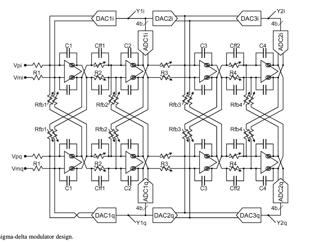
Sigma-Delta examples
There are cool sigma-delta modulators with crazy configurations and that may look like an exercise in “Let’s make something complex”, however, most of them have a reasonable application. One example is the one below for radio recievers
My first Sigma-Delta
The first sigma-delta modulator I made in “real-life” was for the nRF51. The ADC was similar to the one shown below.
The input voltage is translated into a current, and the current is integrated on capacitor $C$. The $R_{offset}$ is to change the mid-level voltage, while $R_{ref}$ is the 1-bit feedback DAC. The comparator is the quantizer. When the clock strikes the comparator compares the $V_o$ and $V_{ref}/2$ and outputs a 1-bit digital output $D$
The complete ADC is operated in a “incremental mode”, which is a fancy way of saying
Reset your sigma-delta modulator, run the sigma delta modulator for a fixed number of cycles (i.e 1024), and count the number of ones at $D$
The effect of an “incremental mode” is to combine the modulator and a output filter so the ADC appears to be a slow Nyquist ADC.
For more information, ask me, or see the patent at Analogue-to-digital converter
