Smith chart plugin
What it does
cicwave-smith is an example plugin for RF work.
It lives in
examples/cicwave-smith
and adds two things to cicwave:
- a reader for Touchstone S-parameter files (
.s1pto.s9p), the format VNAs and RF simulators write; - a Smith chart analysis in the wave context menu.
The UART decoder shows an analysis on its own; this plugin also shows how a reader makes a new file format open like any other.
Trying it
cd examples/cicwave-smith
pip install -e .          # next to an installed cicwave
python make_demo.py       # writes antenna.s1p
cicwave antenna.s1p
make_demo.py models an antenna as a series RLC (35 Ω, resonant at
2.45 GHz, Q = 8) behind 12 mm of 50 Ω feed line, and writes its S11 from
2 to 3 GHz as # GHZ S MA R 50, as a VNA would.
-
The file opens like any other, with a
frequencyx-axis and, for each parameter, the complex value (S11), its magnitude in dB (S11_dB) and its phase (S11_deg). PlottingS11_dBshows the match dip: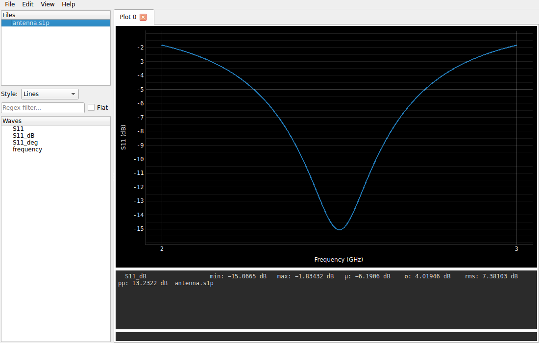
-
Right-click
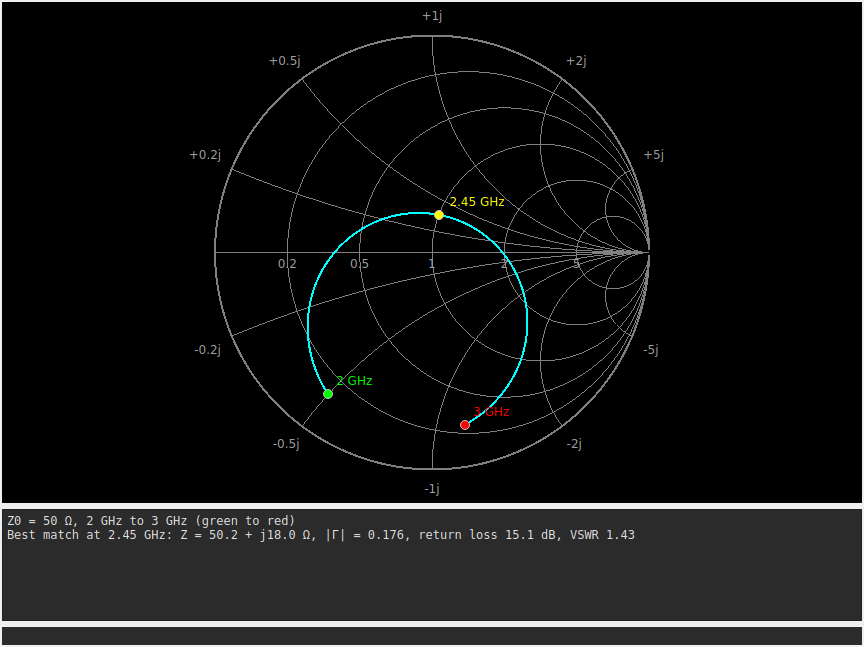
S11, orS11_dB/S11_deg, which map back toS11, and choose Smith chart. A tab opens with the trace on the chart. The first frequency is marked green, the last red, and the best match (smallest |Γ|) yellow. The readout gives the best match’s impedance, return loss and VSWR:Z0 = 50 Ω, 2 GHz to 3 GHz (green to red) Best match at 2.45 GHz: Z = 50.2 + j18.0 Ω, |Γ| = 0.176, return loss 15.1 dB, VSWR 1.43
How a Smith chart works
A load $Z$ on a line of characteristic impedance $Z_0$ reflects part of the incoming wave. The reflection coefficient is
\[\Gamma = \frac{Z - Z_0}{Z + Z_0} = \frac{z - 1}{z + 1}, \qquad z = \frac{Z}{Z_0} = r + jx\]For a one-port, $\Gamma$ is exactly what a VNA measures as $S_{11}$. Any passive load has $r \ge 0$ and so $|\Gamma| \le 1$. The Smith chart is the $\Gamma$ plane, the unit disc, drawn with a grid of impedance rather than $\Gamma$. You can then read a point’s impedance directly and still see how well it is matched.
The grid. The map from $z$ to $\Gamma$ turns straight lines into circles:
- lines of constant resistance $r$ become circles touching the right-hand edge. $r = 0$ is the outer rim and $r = 1$ passes through the centre;
- lines of constant reactance $x$ become arcs from the right-hand edge. Arcs in the upper half ($x > 0$) are inductive and arcs in the lower half ($x < 0$) are capacitive;
- the horizontal axis is pure resistance: a short circuit at the left, $Z_0$ in the centre, an open circuit at the right.
Distance from the centre is mismatch. At the centre, $Z = Z_0$ and nothing is reflected. The further a point is from the centre, the more is reflected:
\[\text{RL} = -20 \log_{10} |\Gamma| \ \text{dB}, \qquad \text{VSWR} = \frac{1 + |\Gamma|}{1 - |\Gamma|}\]Common limits for “matched” are circles around the centre: radius 1/3 is VSWR 2 (9.5 dB return loss), and radius 0.32 is 10 dB return loss.
A feed line rotates the trace. A lossless line of length $\ell$ between the reference plane and the load multiplies $\Gamma$ by $e^{-2j\beta\ell}$, which turns the trace clockwise about the centre without changing $|\Gamma|$. In the demo, that is why the best match (2.45 GHz, the RLC’s resonance) sits above the real axis at $50.2 + j18.0\ \Omega$ rather than on it at 35 Ω. The line changes the impedance seen, not how well it is matched. A resonance appears as a loop, and a larger loop through the centre means a better match.
How it plugs in
register describes the plugin, claims the Touchstone suffixes and adds
the analysis:
def register(api):
    api.set_description("Reads Touchstone .sNp files; draws Smith charts")
    for n in range(1, 10):
        api.register_reader(".s%dp" % n, touchstone.read)
    api.register_analysis("Smith chart", smith_chart)
The reader (cicwave_smith/touchstone.py) is plain numpy and pandas.
It takes the file path and returns a DataFrame. It reads the # option
line (frequency unit, parameter, DB/MA/RI format, reference
resistance), records that wrap over several lines, a 2-port’s special
S11 S21 S12 S22 order, and it stops at the noise block that can follow
a 2-port’s data. $Z_0$ goes in df.attrs['touchstone'], where the
analysis finds it.
The analysis (cicwave_smith/__init__.py) gets the complex column
behind the chosen wave and draws everything into a tab from
window.add_analysis_tab(). Each grid line is a straight line in the
impedance plane, sampled and mapped through $\Gamma = (z-1)/(z+1)$
(smith.grid_lines()), so the chart needs no circle geometry:
t = np.tan(np.linspace(-np.pi / 2, np.pi / 2, n)[1:-1])   # -inf..inf
for r in GRID_R:
    lines.append(("r=%g" % r, gamma_from_z(r + 1j * t, 1.0)))
The tab’s plot is a normal pyqtgraph PlotWidget, with the axes hidden
and the aspect ratio locked so circles stay round.
cicwave’s test suite checks the reader in all three formats, the 2-port
order and noise block, and the chart maths (SmithExampleTest in
tests/unittests/test_plugins.py). screenshots.py in the example
regenerates the pictures on this page.