MOSFETs
If you find an error in what I’ve made, then fork, fix lectures/lr0_mosfet.md, commit, push and create a pull request. That way, we use the global brain power most efficiently, and avoid multiple humans spending time on discovering the same error.
- Metal Oxide Semiconductor
- Field Effect
- Analog transistors in the books
- Transistors in weak inversion
- Transistors in strong inversion
- How should I size my transistor?
- Introduction to behavior
- Weak inversion
- Velocity saturation
- OTHER
- Variability
Status: 0.3
I’m stunned if you’ve never heared the word “transistor”. I think most people have heard the word. What I find funny is that almost nobody understand in full detail how transistors work.
Through my 30 year venture into the world of electronics I’ve met “analog designers”, or people that should understand exactly how transistors work. I used to hire analog designers, and I’ve interviewed hundred plus “analog designers” in my 8 years as manager and I’ve met hundreds of students of analog design. I would go as far as to say none of them know everything about transistors, including myself.
Most of the people I’ve met have a good brain, so that is not the reason they don’t understand. Transistors are incredibly complicated! I say this, because if at some point in this document, you don’t understand, then don’t worry, you are not alone.
In this document I’m focusing on Metal Oxide Semiconductor Field Effect Transistors (MOSFETs), and ignore all other transistors.
Metal Oxide Semiconductor
The first part of the MOSFET name illustrates the 3 dimensional composition of the transistor. Take a semiconductor (Silicon), grow some oxide (Silicon Oxide, SiO2), and place a metal, or conductive, gate on top of the oxide. With those three components we can build our transistor.
Something like the cartoon below where only the Metal (gate) of the MOS name is shown.
The oxide and the silicon bulk is not visible, but you can imagine them to be underneath the gate, with a thin oxide (a few nano meters thick) and the silicon the transparent part of the picture.
The length (L), and width (W) of the MOS is annotated in blue.

Figure 1: 3D crossection of a transistor
MOSFETs come in two main types. There is NMOS, and PMOS. The symbols are as shown below. The NMOS is MN1 and PMOS is MP1.

Figure 2: Transistor symbols
The MOS part of the name can be seen in MN1, where $V_{G}$ is the gate connected to a vertical line (metal), a space (oxide), and another vertical line (the silicon substrate or silicon bulk).
On the sides of the gate we have two connections, a drain $V_{D}$ and a source $V_{S}$.
If we have a sufficient voltage between gate and source $V_{GS}$, then the transistor will conduct from drain to source. If the voltage is too low, then there will not be much current.
The “source” name is because that’s where the charge carrier (electrons) come from, they come from the source, and flow towards the drain. As you may remember, the “current”, as we’ve defined it, flows opposite of the electron current, from drain to source.
The PMOS works in a similar manner, however, the PMOS is made of a different type of silicon, where the dominant charge carrier is holes in the valence band. As a result, the gate-source voltage needs to be negative for the PMOS to conduct.
In a PMOS the holes come from the source, and flow to the drain. Since holes are positive charge carriers, the current flows from source to drain.
In most MOSFETs there is no physical difference between source and drain. If you flip the transistor it would work almost exactly the same.
Field Effect
Imagine that the bulk (the empty space underneath the gate), and the source is connected to 0 V. Assume that the gate is 0 V.
In the source and drain parts of the transistor there is an abundance of free electrons that can move around, exactly like in a metal conductor, however, underneath the gate there are almost no free electrons.
There are electrons underneath the gate though, trillions upon trillions of electrons, but they are stuck in co-valent bonds between the Silicon atoms, and around the nucleus of the Silicon atoms. These electrons are what we call bound electrons, they cannot move, or more precisely, they cannot contribute to current (because they do move, all the time, but mostly around the atoms).
Imagine that your eyes could see the free electrons as a blue fluorescent color. What you would see is a bright blue drain, and bright blue source, but no color underneath the gate.

Figure 3: MOSFET in “off” state
As you increase the gate voltage, the color underneath the gate would change. First, you would think there might be some blue color, but it would be barely noticeable.

Figure 4: MOSFET in subthreshold
At a certain voltage, suddenly, there would be a thin blue sheet underneath the gate. You’d have to zoom in to see it, in reality it’s a ultra thin, 2 dimensional electron sheet.
As you continue to increase the gate voltage the blue color would become a little brighter, but not much.

Figure 5: MOSFET in strong inversion
This thin blue sheet extend from source to drain, and create a conductive channel where the electrons can move from source to drain (or drain to source), exactly like a resistor. The conductance of the sheet is the same as the brightness, higher gate source voltage, more bright blue, higher conductance, less resistance.
Assume you raise the drain voltage. The electrons would move from source to drain proportional to the voltage. How many electrons could move would depend on the gate voltage.
If the gate voltage was low, then there is low density of electrons in the sheet, and low current.
If the gate voltage is high, then the electron density in the sheet is high, and there can be a high current, although, the electrons do have a maximum speed, so at some point the current does not change as fast with the gate voltage.
At a certain drain voltage you would see the blue color disappear close to the drain and there would be a gap in the sheet.

Figure 6: MOSFET in strong inversion and saturation
That could make you think the current would stop, but it turns out, that the electrons close to drain get swept across the gap because the electric field is so high from the edge of the sheet to the drain.
As you continue to increase the drain voltage, the gap increases, but the current does not really increase that much. It’s this exact feature that make transistor so attractive in analog circuits. I can create a current from drain to source that does not depend much on the drain to source voltage! That’s why we sometimes imagine transistors as a “trans-conductance”. The conductance between drain and source depends on the voltage somewhere else, the gate-source voltage.
And now you may think you understand how the transistor works. By changing the gate voltage, we can change the electron current from source to drain. We can turn on, and off, currents, creating a 0 and 1 state.
For example, if I take a PMOS and connect the source to a high voltage, the drain to an output, and an NMOS with the source to ground and the drain to the output, and connect the gates together, I would have the simplest logic gate, an inverter, as shown below.
If the input $V_{in}$ is a high voltage, then the output $V_{out}$ is a low voltage, because the NMOS is on. If the input $V_{in}$ is a low voltage, then the output $V_{out}$ is a high voltage, because the PMOS is on.

Figure 7: Inverter
I can now build more complex “logic gates”. The one below is a Not-AND gate (NAND). If both inputs (A and B) are high, then the output is low (both NMOS are on). Otherwise, the output is high.
I find it amazing that all digital computers in existence can be constructed from the NAND gate. In principle, it’s the only logic gate you need. If you actually did construct computers from NANDs only, they would be costly, and consume lots of power. There are smarter ways to use the transistors.
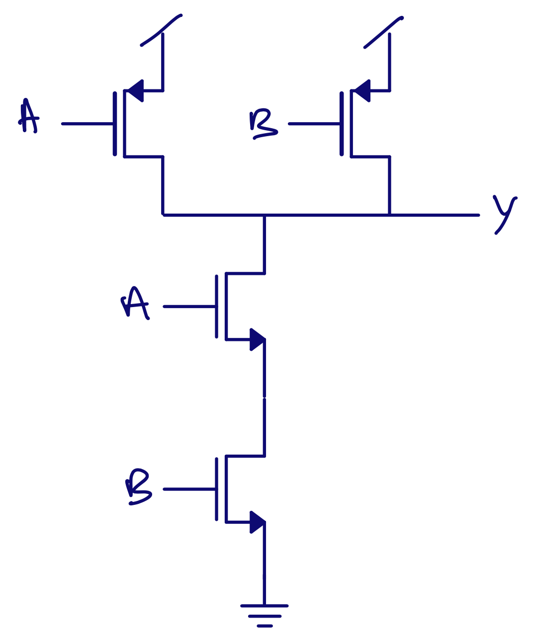
Figure 8: NAND
You may be too young to have seen the Matrix, but now is the time to decide between the red pill and the blue pill.
The red will start your journey to discover the reality behind the transistor, the blue pill will return you to your normal life, and you can continue to think that you now understand how transistors work.
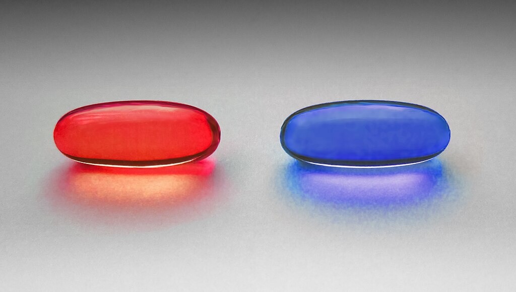
Figure 9: The choice
Because:
- Why did the area underneath the gate turn blue?
- Why is it only a thin sheet that turns blue?
- Where did the electrons for the sheet come from?
- Why did the blue color change suddenly?
- How does the brightness of the blue change with gate-source voltage?
- How can the electrons stay in that sheet when we connect the bulk to 0 V?
- Why is there not a current from the bulk (0 V) to drain?
- Why does not the electrons jump from source to drain? It’s a gap, the same as from the sheet to drain?
And did you realize I never in this chapter explained how the field effect worked?
Someday, I may write all the details, if I ever understand it all. For now, I hope that the sections below will help you a bit.
Analog transistors in the books
In the books we learn the equations for weak inversion
\[I_D \propto (e^{(V_{gs}-V_{th})/U_T}-1)\], where $I_D$ is the drain current, $V_{gs}$ is the gate source voltage, $V_{th}$ is the threshold voltage and $U_T = kT/q$, where $k$ is Boltzmann’s constant, $T$ is the temperature in Kelvin and $q$ is the unit charge
The equation is similar to bipolar and diode equations, because the physics is the same.
The drain current in weak inversion is mostly a diffusion current and relates to the density of electrons in the conduction band (for an NMOS), which can be computed from the density of available energy states, and the Fermi-Dirac distribution.
\[n = \int_{E_C}^{\infty}N(E)\frac{1}{e^{(E-E_F)/kT}+1}dE\], where $n$ is the density of electrons in the conduction band, $N(E)$ is the density of available energy states, $E$ is the integration variable (and the energy) and $E_F$ is the Fermi-level.
Maybe the equation looks complicated, but it’s really “Multiply the available energy state with the probability of being in that state, and sum for all available energy states”.
Changing the voltage changes the number of free electrons, simply because we bring the conduction band closer to the Fermi level.
The Fermi level is just something we invented, and just means “If there was an quantum state at the Fermi level Energy, then it would have a 50 % probability of being occupied by a electron”.
In the equation above, moving the conduction band edge is equivalent to reducing the $E_C$. As such, more of the Fermi-Dirac distribution has available energy states $N(E)$, and the density of electrons $n$ in conduction band becomes higher.
In strong inversion, the MOSFET is more like a voltage controlled resistor with a conductance that is proportional to gate-source voltage.
The density of electrons increases because we bend the conduction band beyond the Fermi level, as a result, most of the available energy states in the conduction band are filled by electrons.
Electrons are only free to move, however, close to the surface of the silicon, as far away from the surface, we don’t feel the effects of the gate-source voltage, and the conduction band stays at the same energy. As a result, electrons form a 2 dimensional electron gas close to the silicon surface. What we call an inversion layer.
Once we have that electron gas, or inversion layer, we have a connection between the drain and source n-type regions, and the current can be estimated by a drift current. Parts of the diffusion current will still be there, but much smaller magnitude than the drift current, so we drop the diffusion current, and get
\[I_D = \frac{1}{2} \mu_n C_{ox}\frac{W}{L}(V_{gs}-V_{th})^2\]The equations in the books are good to give a physical understanding of what happens. Although, we tend to forget that everybody forgets.
We teach quantum physics one year, and how to compute the density of states $N(E)$ from Schrodinger, the wave-function and Fermi-Dirac distribution.
Next year we talk about semiconductors, crystal lattice, band structure (density of states as a function of space), energy diagrams (band structure is complex, so we just use the lowest conduction band and highest valence band), doping to shift the Fermi level, and how we can create PN-junctions, bipolars and MOSFETS.
The year after we teach the current equations for MOSFETs, and the books don’t have the link back to solid-state physics, after all, we already told the students that, they should remember!
I think, quite often, we just end up with confused students. And I don’t think it’s necessary to end up with confused students. Maybe sometimes we end up with confused students because the Professors can’t necessarily remember where the equations come from either, nor how electrons and holes really behave.
It’s not necessary for an analog design student to remember how to compute the density of available energy states from Schrodinger and the wave function. If we wanted to use the relativistc version of Schrodinger (which includes magnetic fields, and if you did not know, magnetic fields is just a relativistic effect of the electric field) and the wave function to compute how an Silicon atom actually behaves, I don’t think we can. As far as I’ve been able to figure out, it’s not possible to have a closed form solution (symbolic), nor is it possible with supercomputers to do a numeric time-evolution of the states in a single Silicon atom with all the inter-particle interactions, space, momentum, spins, electric fields and magnetic fields.
But we can make sure we connect the links from Schrodinger to the MOSFET equations, the short version of that was above, but the following sections tries to explain with words how the transistor actually works.
I’m not going to give all the equations and all the maths. For that, there are excelent books and resources. I would recommend Mark Lundstrom for the best in detail description of MOSFETs.
Transistors in weak inversion
Consider the cartoon below which shows the hole concentration in the valence band, and electron concentration in the conduction band versus the x direction of the transistor.
For the moment we’ll ignore the field effect of the gate, and how that modulates the hole concentration underneath the gate.
If you’re familiar with bipolars, then you may think I’ve drawn the wrong transistor, because you see an NPN bipolar transistor. The picture is correct, however, this is how a normal MOSFET looks. It’s actually also a NPN bipolar transistor, but we don’t usually use that part (you’ll see more when we get to ESD)
In the source we’ve doped with donors, and have an abundance of free electrons. Underneath the gate, or the bulk, we have doped with acceptors, and have an abundance of holes.

Figure 10: Charge carrier density in a MOSFET
Let’s consider electron current for now, and only look at the conduction band.
An electron in the source would see a energy barrier of $\phi_B$, and most electrons would be turned around at the barrier. Some, however, do have the energy to traverse the barrier and flow through the bulk. Not all of them would reach the bulk, due to recombination, but let’s assume the bulk is short, and all electrons injected into the bulk show up at the drain.
At the drain side they would fall down the potential barrier to the drain. The same process would happen in reverse, from drain to source.

Figure 11: MOSFET subthreshold , $V_{DS} = 0$
There would also be hole currents flowing between source/bulk/drain and visa versa
Assume source and drain are at the same potential, then the sum of all currents (1,2,3,4) for both electrons and holes in Figure 11 must equal zero.
Assume that we increase the drain voltage, as shown in Figure 12. Increasing the drain voltage is the same as reducing the conduction band in the drain.
Since there now is a higher barrier from drain to bulk, it’s now much less probable that electrons are injected from drain to bulk.
Now the sum of all currents would not equal zero, as the 1 and 3 currents are larger than 2 and 4.
As such, there would be a net flow of electron current from source to drain.

Figure 12: MOSFET subthreshold, $V_{S} = 0\text{ V}, V_D > 0\text{ V}$
Notice that if we increase the drain voltage further, then the electron injection from drain to bulk would quickly approach zero.
At that point, even though we increase the drain voltage further, the current does not really change. As the current is only now given by the barrier height at the source.
The barrier height at the source is the built in voltage of the junction, and as we’ve seen before, that voltage depends on doping concentration. If we increase the hole concentration in bulk, then we increase the barrier height, and it’s less probable that the electrons have enough energy to be injected from source to bulk.
If we only need to consider the electrons and holes at source for the subthreshold current (assuming the drain voltage is high enough), then we should expect the equation look very similar to a diode, and indeed it does.
The drain current, which is mostly a diffusion current, is given by
\[I_{D} = I_{D0} \frac{W}{L} e^{q(V_{GS} - V_{TH})/ n kT}\]where
\[n = (C_{ox} + C_{j0})/C_{ox}\] \[I_{D0} = (n - 1) \mu_n C_{ox} \left(\frac{kT}{q}\right)^2\]This is not exactly the same as the diode equation, but we can see that it looks similar. Most of the quantum mechanics is baked into the $V_{TH}$
The transconductance ($dI_D/dV_{GS}$) in weak inversion is then
\[g_m = \frac{I_D}{nV_T}\]A big difference from the diode equation is the fact that the gate-source voltage seems to determine the current, and not the voltage across the pn junction.
Transistors in strong inversion
Consider the band diagram in Figure 13, in the figure we’re looking at a cross section of the transistor. From left we’re in the gate, then we have the oxide, and then the bulk of the transistor.
We don’t see the drain and source, as the source would be towards you, and the drain would be into the picture.
The cartoon is not a real transistor. I don’t think there is necessarily a combination of semiconductor and metal where we end up with the same Fermi level ($E_F$) without some bending of the conduction band and valence band, but for illustration, let’s assume that’s the case.
We can see the Fermi level in the semiconductor is shifted towards the valence band, and thus we have a P-type semiconductor.
The gate is metallic, so it does not have a bandgap, and we assume that the Fermi level is at the conduction band edge.

Figure 13: Band diagram of a fictive MOSFET.
Assume we increase the gate-source voltage. In a band diagram that corresponds to shifting the energy down.

Figure 14: Band diagram with gate-source voltage applied
Moving the gate down has the effect of bending the bands in the semiconductor. We’ll lose some voltage across the oxide, but not necessarily that much.
The bending of the valence band will decrease the hole concentration close to the silicon surface, and the semiconductor will be depleted of mobile charge carriers.
The valence band bending will also reduce the barrier height in Figure 12, which increases the number of carriers that can be injected at source/bulk interface, so the subthreshold current will start to increase.
At some point, the band bending of the conduction band will become so large that the electron concentration underneath the gate will increase signficantly. The gate-source voltage where the electron concentration equals the bulk hole concentration far away from the silicon surface is called the “threshold voltage”.
As you continue to increase the gate-source voltage there is a limit to how much the electron concentration increases. When the band bending of the conduction band passes the Fermi level, then over 50 percent of the available states in the conduction band are filled with electrons.

Figure 13: Band diagram with high gate-source voltage applied
The conditions to be in strong inversion is that the gate/source voltage is above some magic values (threshold voltage), and then some.
The quantum state of the electron is fully determined by it’s spin, momentum and position in space. How those parameters evolve with time is determined by the Schrodinger equation. In the general form
\[i\hbar\frac{d}{dt}\Psi(r,t) = \widehat{H} \Psi(r,t)\]The Hamiltonian ($H$) is an “energy matrix” operator and may contain terms both for the momentum and Columb force (electric field) experienced by the system.
But what does the Schrodinger equation tell us? Well, the equation above does not tell me much, it can’t be “solved”, or rather, it does not have a single solution. It’s more a framework for how the wave function, and the Hamiltonian, describes the quantum states of a system, and the probability ampltiudes of transition between states.
The Schrodinger equation describes the time evolution of the bound electrons shared between the Silicon atoms, and the fact that applying a electric field to silicon can free co-valent bonds.
As the gate-source voltage increases the wave function that fits in the Schrodinger equation predicts that the free electrons will form a 2d sheet underneath the gate. The thickness of the sheet is only a few nano meters.
In Figure 2 in
Carrier transport near the Si/SiO2 interface of a MOSFET
you can see how the free electron density is located underneath the gate.
I would really recommend that you have a look at Mark Lundstrom’s lecture series on Essentials of MOSFETs. It’s the most complete description of electrons in MOSFET’s I’ve seen
How should I size my transistor?
The method that makes most sense to me, is to use the inversion-coefficient method, described in Nanoscale MOSFET Modeling: Part 1 and Nanoscale MOSFET Modeling: Part 2.
The inversion coefficient tells us how strongly inverted the MOSFET channel (inversion layer) is. A number below 0.1 is weak inversion, between 0.1 and 10 is moderate inversion. A number above 10 is strong inversion.
There are also some blog posts worth looking at Inversion Coefficient Based Circuit Design and My Circuit Design Methodology.
I should caveat my proposal for method. For the past 7 years I’ve not had the luxury to do full time, hardcore, analog design. As my career progressed, most of my time is now spent telling others what I think is a good idea to do, and not doing hardcore analog design myself. I think, however, I have a pretty decent understanding of analog circuits, and how to design them, so I think I’m correct in the proposal. If I were to start hardcore analog design now, I would go all in on inversion-coefficient based transistor size selection.
Introduction to behavior
Let’s assume we know nothing about how transistors work, but we do know how to simulate them in ngspice.
We could sit down, and try and figure out how the transistors work.
You can find the testbenches at Testbenches at dicex/sim/spice/NCHIO
Drain Source Current
Let’s see what happens to the drain to source current when we change the voltages. We would expect the drain to source current to change as a function of the drain to source, $V_{DS}$, and gate to source $V_{GS}$ voltages. Or mathematically
\[I_{DS} = f(V_{GS},V_{DS},...)\]or symbolically

The symbolic model above is what we call a “Large Signal Model”. We could expand the function above to
\[I_{DS} = f(V_{GS},V_{DS}) = G_m(V_{GS},V_{DS},I_{DS}) V_{GS} + G_{ds}(V_{GS},V_{DS},I_{DS}) V_{DS}\], where the $G_m$ is a trans-conductance (the current depends on a voltage somewhere else), and $G_{ds}$ is a conductance (current depends on the voltage across the conductance).
Even now we can see that the model above is complicated. The transconductance and conductance of the transistor is a function of the other voltages, and the output current. It’s a non-linear system!
If the transistor was linear, then we would expect that the current increased proportionally to gate/source voltage, but how does the current look when we change the gate source voltage?
Gate-source voltage
Below are the conditions I’ve used in the testbench. Notice there is a $V_{B}$ that is the $p-$ substrate, or bulk, of the transistor. When we draw symbols of a transistor we don’t always include the bulk node, because that’s most of the time connected to ground for NMOS.
But sometimes, we connect the bulk to another voltage, so the bulk terminal will be in our schematics.
| Param | Voltage |
|---|---|
| VGS | 0 to 1.8 |
| VDS | 1.0 |
| VS | 0 |
| VB | 0 |
In the plot below we can see the sweep of the gate voltage.
\[i(vcur) = I_{DS}\]
Inversion level
Define \(V_{eff} \equiv V_{GS} - V_{tn}\) , where \(V_{tn}\) is the “threshold voltage”
| Veff | Inversion level |
|---|---|
| less than 0 | weak inversion or subthreshold |
| 0 | moderate inversion |
| more than 100 mV | strong inversion |
Weak inversion
The drain current is low, but not zero, when
\[V_{eff} << 0\] \[I_{DS} \approx I_{D0} \frac{W}{L} e^{V_{eff}/n V_{T}} \text{ if } V_{DS} > 3 V_{T}\] \[n \approx 1.5\]Moderate inversion
Very useful region in real designs. Hard for hand-calculation. Trust the model.
Strong inversion
\[I_{DS} = \mu_n C_{ox} \frac{W}{L} \begin{cases} V_{eff} V_{DS} & \text{if }V_{DS} << V_{eff} \\[15pt] V_{eff} V_{DS} - V_{DS}^2/2 & \text{if } V_{DS} < V_{eff} \\[15pt] \frac{1}{2} V_{eff}^2 & \text{if } V_{DS} > V_{eff} \\[15pt] \end{cases}\]


Drain source voltage
| Param | Voltage [V] |
|---|---|
| VGS | 0.5 |
| VDS | 0 to 1.8 |
| VS | 0 |
| VB | 0 |

Strong inversion
\[I_{DS} = \mu_n C_{ox} \frac{W}{L} \begin{cases} V_{eff} V_{DS} & \text{if }V_{DS} << V_{eff} \\[15pt] V_{eff} V_{DS} - V_{DS}^2/2 & \text{if } V_{DS} < V_{eff} \\[15pt] \frac{1}{2} V_{eff}^2 & \text{if } V_{DS} > V_{eff} \\[15pt] \end{cases}\]


Low frequency model
\[g_{m} = \frac{\partial I_{DS}}{\partial V_{GS}}\] \[g_{ds} = \frac{1}{r_{ds}} = \frac{\partial I_{DS}}{\partial V_{DS}}\]
Transconductance
Define \(\ell = \mu_n C_{ox} \frac{W}{L}\) and \(V_{eff} = V_{GS} - V_{tn}\)
\(I_{D} = \frac{1}{2} \ell (V_{eff})^2\) and \(V_{eff} = \sqrt{\frac{2I_{D}}{\ell}}\) and \(\ell = \frac{2I_D}{V_{eff}^2}\)
\[g_m = \frac{ \partial I_{DS}} {\partial V_{GS}} = \ell V_{eff} = \sqrt{2 \ell I_{D}}\] \[g_m = \ell V_{eff} = 2 \frac{I_D}{V_{eff}^2} V_{eff} = \frac{2 I_D}{V_{eff}}\]Define \(\ell = \mu_n C_{ox} \frac{W}{L}\) and \(V_{eff} = V_{GS} - V_{tn}\)
\[I_D = \frac{1}{2} \ell V_{eff}^2[1 + \lambda V_{DS} - \lambda V_{eff})]\] \[\frac{1}{r_{ds}} = g_{ds} = \frac{ \partial I_D}{\partial V_{DS} } = \lambda \frac{1}{2} \ell V_{eff}^2\]Assume channel length modulation is not there, then
\(I_D = \frac{1}{2} \ell V_{eff}^2\) which means \(\frac{1}{r_{ds}} = g_{ds} \approx \lambda I_D\)
Intrinsic gain
Define intrinsic gain as
\[A = \left|\frac{v_{out}}{v_{in}}\right| = g_m r_{ds} = \frac{g_m}{g_{ds}}\] \[A = \frac{2 I_D}{V_{eff}} \times \frac{1}{ \lambda I_D } = \frac{2}{\lambda V_{eff}}\]
vgaini = Gate Source Voltage = \(V_{eff} + V_{tn}\)

High frequency model


\(C_{gs}\) and \(C_{gd}\)
\[C_{gs} = \begin{cases} WLC_{ox} & \text{if }V_{DS} = 0 \\[15pt] \frac{2}{3}WLC_{ox} & \text{if }V_{DS} > V_{eff} \\[15pt] \end{cases}\] \[C_{gd} = C_{ox} W L_{ov}\]\(C_{sb}\) and \(C_{db}\)
Both are depletion capacitances
\[C_{sb} = (A_s + A_{ch}) C_{js}\] \[C_{js} = \frac{C_{j0}}{\sqrt{1 + \frac{V_{SB}}{\Phi_0}}}\] \[\Phi_0 = V_T ln\left(\frac{N_A N_D}{n_i^2}\right)\] \[C_{db} = A_d C_{jd}\] \[C_{js} = \frac{C_{j0}}{\sqrt{1 + \frac{V_{DB}}{\Phi_0}}}\]Be careful with Cgd (blame Miller)
If \(Y(s) = 1/sC\) then \(Y_1(s) = 1/sC_{in}\) and \(Y_2(s) = 1/sC_{out}\) where \(C_{in} = (1 + A) C\), \(C_{out} = (1 + \frac{1}{2})C\)
\[C_{1} = C_{gd} g_{m} r_{ds}\]\(C_{gd}\) can appear to be 10 to 100 times larger!
if gain from input to output is large

Weak inversion
If \(V_{eff} < 0\) diffusion currents dominate.
\(I_{D} = I_{D0} \frac{W}{L} e^{V_eff / n V_T}\), where
\(V_T = kT/q\), \(n = (C_{ox} + C_{j0})/C_{ox}\)
\[I_{D0} = (n - 1) \mu_n C_{ox} V_T^2\] \[g_m = \frac{I_D}{nV_T}\]
Bang for the buck
Subthreshold:
\[\frac{g_m}{I_D} = \frac{1}{nV_T} \approx 25.6 \text{ [S/A] @ 300 K}\]Strong inversion:
\[\frac{g_m}{I_D} = \frac{2}{V_{eff}}\]
Velocity saturation
Electron speed limit in silicon
\[v \approx 10^7 cm/s\] \[v = \mu_n E = \mu_n \frac{dV}{dx}\]\(\mu_n \approx 100 \text{ to } 600 \text{ } cm^2/Vs\) in nanoscale CMOS

Square law model
\[Q(x) = C_{ox}\left[V_{eff} - V(x)\right]\] \[v = \mu_n E = \mu_n \frac{dV}{dx}\] \[\ell = \mu_n C_{ox} \frac{W}{L}\] \[I_{D} = W Q(x) v = \ell L \left[ V_{eff} - V(x)\right] \frac{dV}{dx}\] \[I_{D} dx = \ell L \left[ V_{eff} - V(x)\right] dV\] \[I_{D} \int_0^L{dx} = \ell L \int_0^{V_{DS}}{\left[ V_{eff} - V(x)\right] dV}\] \[I_{D} \left[x\right]_0^L = \ell L \left[V_{eff}V - \frac{1}{2}V^2\right]_0^{V_{DS}}\] \[I_{D} L = \ell L \left[V_{eff}V_{DS} - \frac{1}{2} V_{DS}^2\right]\] \[@ V_{DS} = V_{eff} \Rightarrow I_{D} = \frac{1}{2} \ell V_{eff}^2\]Mobility Degradation
Multiple effects degrade mobility
- Velocity saturation
- Vertical fields reduce channel depth => more charge-carrier scattering
From square law \(g_{m} = \frac{\partial I_{D}}{\partial V_{GS}} = \ell V_{eff}\)
With mobility degradation \(g_{m(mob-deg)} = \frac{\ell}{2 \theta}\)
What about holes (PMOS)
In PMOS holes are the charge-carrier (electron movement in valence band)
\[\mu_p < \mu_n\]In intrinsic silicon: \(\mu_n \leq 1400 [cm^2/Vs] = 0.14 [m^2/Vs]\) \(\mu_p \leq 450 [cm^2/Vs] = 0.045 [m^2/Vs]\)
\[\mu_n \approx 3\mu_p\]\(v_{n\_max} \approx 2.3 \times 10^5 [m/s]\) \(v_{p\_max} \approx 1.6 \times 10^5 [m/s]\)
Doping (\(N_A \text{or} N_D\)) reduces \(\mu\)
OTHER
As we make transistors smaller, we find new effects that matter, and that must be modeled.
which is an opportunity for engineers to come up with cool names
https://ieeexplore.ieee.org/document/5247174

Drain induced barrier lowering (DIBL)

Well Proximity Effect (WPE)

Stress effects
| Stress | PMOS | NMOS |
|---|---|---|
| Stretch Fz | Good | Good |
| Compress Fy | OK | Good |
| Compress Fx | Good | Bad |
What can change stress?

Gate current

Hot carrier injection

Channel initiated secondary-electron (CHISEL)

Variability
Provide \(I_2 = 1 \mu A\)
Let’s use off-chip resistor \(R\), and pick \(R\) such that \(I_1 = 1 \mu A\)
Use \(\frac{W_1}{L_1} = \frac{W_2}{L_2}\)
What makes \(I_2 \ne 1 \mu A\)?

- Voltage variation
- Systematic variations
- Process variations
- Temperature variation
- Random variations
- Noise
Voltage variation
\[I_1 = \frac{V_{DD} - V_{GS1}}{R}\]If \(V_{DD}\) changes, then current changes.
Fix: Keep \(V_{DD}\) constant
Systematic variations
If \(V_{DS1} \ne V_{DS2} \rightarrow I_1 \ne I_2\)
If layout direction of \(M_1 \ne M_2 \rightarrow I_1 \ne I_2\)
If current direction of \(M_1 \ne M_2 \rightarrow I_1 \ne I_2\)
If \(V_{S1} \ne V_{S2} \rightarrow I_1 \ne I_2\)
If \(V_{B1} \ne V_{B2} \rightarrow I_1 \ne I_2\)
If \(WPE_{1} \ne WPE_{2} \rightarrow I_1 \ne I_2\)
If \(Stress_{1} \ne Stress_{2} \rightarrow I_1 \ne I_2\) …
Process variations
Assume strong inversion and active \(V_{eff} = \sqrt{\frac{2}{\mu_p C_{ox} \frac{W}{L}} I_1}\), \(V_{GS} = V_{eff} + V_{tp}\)
\[I_1 = \frac{V_{DD} - V_{GS}}{R} = \frac{V_{DD} - \sqrt{\frac{2}{\mu_p C_{ox} \frac{W}{L}} I_1} - V_{tp}}{R}\]\(\mu_p\), \(C_{ox}\), \(V_{tp}\) will all vary from die to die, and wafer lot to wafer lot.
Process corners
Common to use 5 corners, or Monte-Carlo process simulation
| Corner | NMOS | PMOS |
|---|---|---|
| Mtt | Typical | Typical |
| Mss | Slow | Slow |
| Mff | Fast | Fast |
| Msf | Slowish | Fastish |
| Mfs | Fastish | Slowish |
Fix process variation
Use calibration: measure error, tune circuit to fix error
For every single chip, measure voltage across known resistor \(R_1\) and tune \(R_{var}\) such that we get \(I_1 = 1 \mu A\)
Be careful with multimeters, they have finite input resistance (approximately 1 M\(\Omega\))
Temperature variation
Mobility decreases with temperature
Threshold voltage decreases with temperature.
\[I_D = \frac{1}{2}\mu_n C_{ox} (V_{GS} - V_{tn})^2\]High \(I_D =\) fast digital circuits
Low \(I_D =\) slow digital circuits
What is fast? High temperature or low temperature?
It depends on \(V_{DD}\)
Fast corner
- Mff (high mobility, low threshold voltage)
- High \(V_{DD}\)
- High or low temperature
Slow corner
- Mss (low mobility, high threshold voltage)
- Low \(V_{DD}\)
- High or low temperature
How do we fix temperature variation?
Accept it, or don’t use this circuit.
If you need stability over temperature, use 7.3.2 and 7.3.4 in CJM (SUN_BIAS_GF130N)
Random Variation
\[\ell = \mu_p C_{ox} \frac{W}{L}\] \[I_D = \frac{1}{2} \ell (V_{GS} - V_{tp})^2\]Due to doping , length, width, \(C_{ox}\), \(V_{tp}\), … random varation
\[\ell_1 \ne \ell_2\] \[V_{tp1} \ne V_{tp2}\]As a result \(I_1 \ne I_2\), but we can make them close.
Pelgrom’s1 law
Given a random gaussian process parameter \(\Delta P\) with zero mean, the variance is given by
\[\sigma^2 (\Delta P) = \frac{A^2_P}{WL} + S_{P}^2 D^2\]where \(A_P\) and \(S_P\) are measured, and \(D\) is the distance between devices
Assume closely spaced devices (\(D \approx 0\)) \(\Rightarrow \sigma^2 (\Delta P) = \frac{A^2_P}{WL}\)
Transistors with same \(V_{GS}\)2
\[\frac{\sigma_{I_D}^2}{I_D^2} = \frac{1}{WL}\left[\left(\frac{gm}{I_D}\right)^2 \sigma_{vt}^2 + \frac{\sigma_{\ell}^2}{\ell}\right]\]Valid in weak, moderate and strong inversion
\(\frac{\sigma_{I_D}^2}{I_D^2} = \frac{1}{WL}\left[\left(\frac{gm}{I_D}\right)^2 \sigma_{vt}^2 + \frac{\sigma_{\ell}^2}{\ell}\right]\) \(\frac{\sigma_{I_D}}{I_D} \propto \frac{1}{\sqrt{WL}}\)
Assume \(\frac{\sigma_{I_D}}{I_D} = 10\%\), We want \(5\%\), how much do we need to change WL?
\[\frac{\frac{\sigma_{I_D}}{I_D}}{2} \propto \frac{1}{2\sqrt{WL}} = \frac{1}{\sqrt{4WL}}\]We must quadruple the area to half the standard deviation
\(1 \%\) would require 100 times the area

What else can we do?
\[\frac{\sigma_{I_D}^2}{I_D^2} = \frac{1}{WL}\left[\left(\frac{gm}{I_D}\right)^2 \sigma_{vt}^2 + \frac{\sigma_{\ell}^2}{\ell}\right]\]Strong inversion \(\Rightarrow \frac{gm}{I_D} = \frac{1}{2 V_{eff}} = low\)
Weak inversion \(\Rightarrow \frac{gm}{I_D} = \frac{q}{n k T} \approx 25\)
Current mirrors achieve best matching in strong inversion
\[\frac{\sigma_{I_D}^2}{I_D^2} = \frac{1}{WL}\left[\left(\frac{gm}{I_D}\right)^2 \sigma_{vt}^2 + \frac{\sigma_{\ell}^2}{\ell}\right]\] \[\sigma_{I_D}^2 = \frac{1}{WL}\left[gm^2 \sigma_{vt}^2 + I_D^2\frac{\sigma_{\ell}^2}{\ell}\right]\]Offset voltage for a differential pair
\[i_o = i_{o+} - i_{o-} = g_m v_i = g_m (v_{i+} - v_{i-})\] \[\sigma_{v_i}^2 = \frac{\sigma_{I_D}^2}{gm^2} = \frac{1}{WL}\left[\sigma_{vt}^2 + \frac{I_D^2}{gm^2}\frac{\sigma_{\ell}^2}{\ell}\right]\]High \(\frac{gm}{I_D}\) is better (best in weak inversion)

Transistor Noise
Thermal noise Random scattering of carriers, generation-recombination in channel? \(PSD_{TH}(f) = \text{Constant}\)
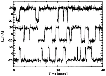
Popcorn noise Carriers get “stuck” in oxide traps (dangling bonds) for a while. Can cause a short-lived (seconds to minutes) shift in threshold voltage \(PSD_{GR}(f) \propto \text{Lorentzian shape} \approx \frac{A}{1 + \frac{f^2}{f_0}}\)
Flicker noise Assume there are many sources of popcorn noise at different energy levels and time constants, then the sum of the spectral densities approaches flicker noise. \(PSD_{flicker}(f) \propto \frac{1}{f}\)