TFE4188 - Lecture 6

Oversampling and Sigma-Delta ADCs

1

Goal for today

Understand why there are different ADCs

Introduction to oversampling and delta-sigma modulators

A few examples

2

1999, R. Walden: Analog-to-digital converter survey and analysis [@walden99]

3

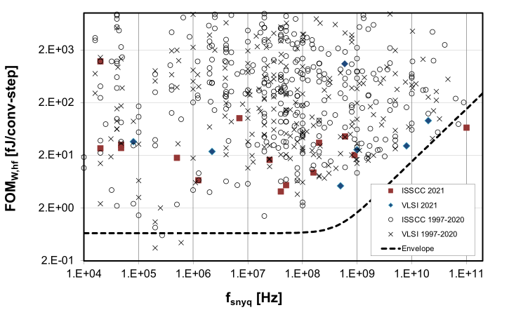
B. Murmann, ADC Performance Survey 1997-2023

\(FOM_W = \frac{P}{2^{ENOB} f_s}\)

Below 10 fJ/conv.step is good.

Below 1 fJ/conv.step is extreme.

4

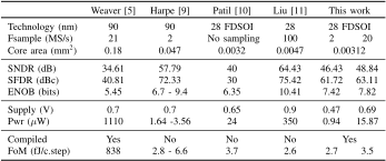
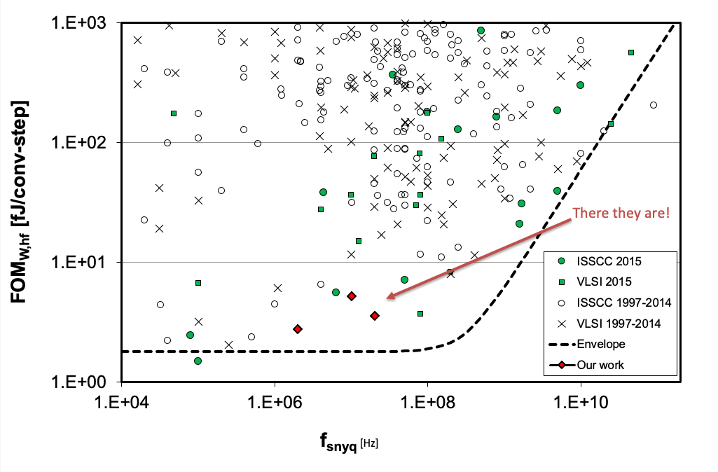
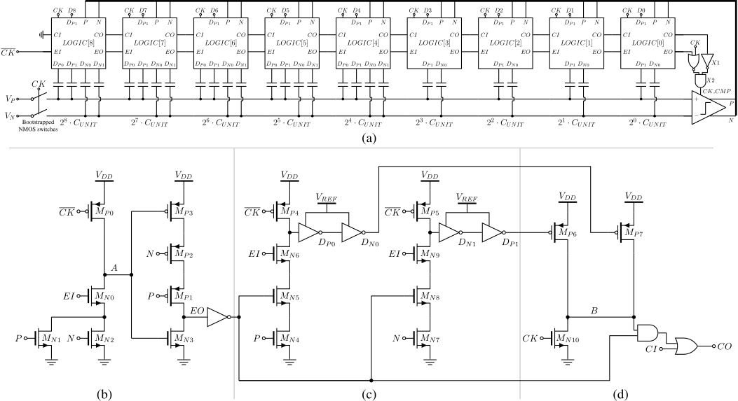
People from NTNU have made some of the world's best ADCs

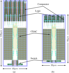
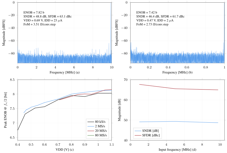
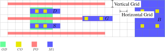
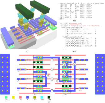
[1] A Compiled 9-bit 20-MS/s 3.5-fJ/conv.step SAR ADC in 28-nm FDSOI for Bluetooth Low Energy Receivers [@wulff17]

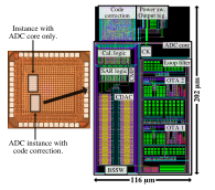
[2] A 68 dB SNDR Compiled Noise-Shaping SAR ADC With On-Chip CDAC Calibration

5

What makes a state-of-the-art ADC

6

7

8

9

10

11

12

13

14

SUN_SAR9B_SKY130NM

15

16

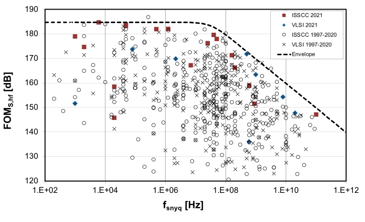
B. Murmann, ADC Performance Survey 1997-2022 (ISSCC & VLSI Symposium)

\(FOM_S = SNDR + 10\log\left(\frac{f_s/2}{P}\right)\)

Above 180 dB is extreme

17

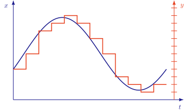
Quantization

18

19

20

21

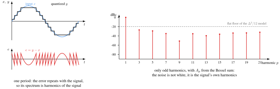
See The intermodulation and distortion due to quantization of sinusoids [@blachman85a] for details

y(t) = \sum_{p=1}^\infty{A_p\sin{p\omega t}}

where p is the harmonic index, and

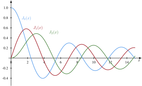
A_p = \begin{cases} \delta_{p1}A + \sum_{m = 1}^\infty{\frac{2}{m\pi}J_p(2m\pi A)} &, p = \text{ odd} \\ 0 &, p = \text{ even} \end{cases}

\delta_{p1} \begin{cases} 1 &, p=1 \\ 0 &, p \neq 1 \end{cases}

and \(J_p(x)\) is a Bessel function of the first kind, A is the amplitude of the input signal.

If we approximate the amplitude of the input signal as

A = \frac{2^n - 1}{2} \approx 2^{n-1}

where n is the number of bits, we can rewrite as

22

y(t) = \sum_{p=1}^\infty{A_p\sin{p\omega t}}

A_p = \delta_{p1}2^{n-1} + \sum_{m=1}^\infty{\frac{2}{m\pi}J_p(2m\pi 2^{n-1})}, p=odd

23

24

25

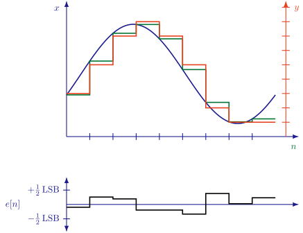
\overline{e_n(t)} = 0

\overline{e_n(t)^2} = \frac{\Delta^2}{12}

26

SQNR = 10 \log\left(\frac{A^2/2}{\Delta^2/12}\right) = 10 \log\left(\frac{6 A^2}{\Delta^2}\right)

\Delta = \frac{2A}{2^B}

SQNR = 10 \log\left(\frac{6 A^2}{4 A^2/2^{2B}}\right) = 20 B \log 2 + 10 \log 6/4

SQNR \approx 6.02 B + 1.76

27

28

29

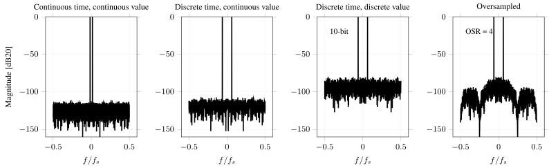
Oversampling

30

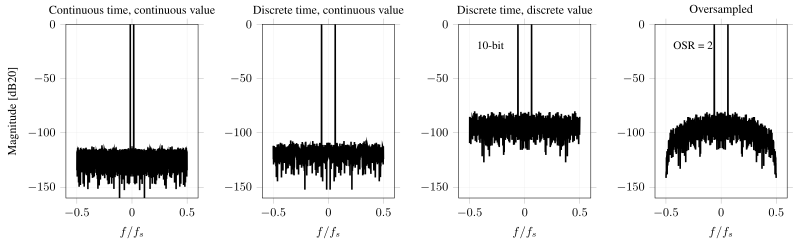
in-band quantization noise for an oversampling ratio (OSR)

\overline{e_n(t)^2} =\frac{\Delta^2}{12 OSR}

SQNR = 10 \log\left(\frac{6 A^2}{\Delta^2/OSR}\right) = 10 \log\left(\frac{6 A^2}{\Delta^2}\right) + 10 \log(OSR)

\(SQNR \approx 6.02B + 1.76 + 10 \log(OSR)\)

10 \log(2) \approx 3 dB

10 \log(4) \approx 6 dB

0.5-bit per doubling of OSR

31

def oversample(x,OSR):
    N = len(x)
    y = np.zeros(N)

    for n in range(0,N):
        for k in range(0,OSR):
            m = n+k
            if (m < N):
                y[n] += x[m]
    return y

32

33

34

Noise Shaping

35

36

37

Sample domain

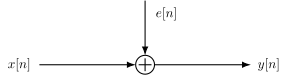
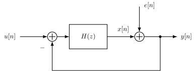
\[y[n] = e[n] + h*(u[n] - y[n])\]

Z-Domain

Y(z) = E(z) + H(z)\left[U(z) - Y(z)\right]

38

Signal transfer function

Assume U and E are uncorrelated, and E is zero

\(Y = HU - HY\)

STF = \frac{Y}{U} = \frac{H}{1 + H} = \frac{1}{1 + \frac{1}{H}}

Noise transfer function

Assume U is zero

Y = E - HY \rightarrow NTF = \frac{1}{1 + H}

39

Combined transfer function

\[Y(z) = STF(z) U(z) + NTF(z) E(z)\]

40

First-Order Noise-Shaping

41

H(z) = \frac{1}{z-1}

STF = \frac{1/(z-1)}{1 + 1/(z-1)} = \frac{1}{z} = z^{-1}

NTF = \frac{1}{1 + 1/(z-1)} = \frac{z-1}{z} = 1 - z^{-1}

42

z = e^{sT} \;\underset{s=j\omega}{\longrightarrow}\; e^{j\omega T} = e^{j2 \pi f/f_s}

\begin{aligned} NTF(f) &= 1- e^{-j2 \pi f/f_s} \\ &= \frac{e^{j \pi f/f_s} -e^{-j \pi f/f_s}}{2j}\times 2j \times e^{-j\pi f/f_s} \\ &= \sin\left(\frac{\pi f}{f_s}\right) \times 2j \times e^{-j \pi f/f_s} \end{aligned}

\vert NTF(f)\vert = \left\vert 2 \sin\left(\frac{\pi f}{f_s}\right)\right\vert

43

\[P_s = A^2/2\]

P_n = \int_{-f_0}^{f_0} \frac{\Delta^2}{12}\frac{1}{f_s}\left[2 \sin\left(\frac{\pi f}{f_s}\right)\right]^2 df

\(SQNR = 6.02 B + 1.76 - 5.17 + 30 \log(OSR)\)

44

SQNR and ENOB

\(SQNR_{nyquist} \approx 6.02B + 1.76\)

\(SQNR_{oversample} \approx 6.02B + 1.76 + 10 \log(OSR)\)

\(SQNR_{\Sigma\Delta 1} \approx 6.02 B + 1.76 - 5.17 + 30 \log(OSR)\)

SQNR_{\Sigma\Delta 2} \approx 6.02 B + 1.76 - 12.9 + 50 \log(OSR)

\[ENOB = (SQNR - 1.76)/6.02\]

45

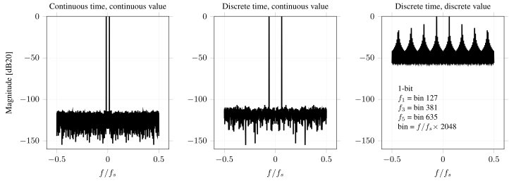
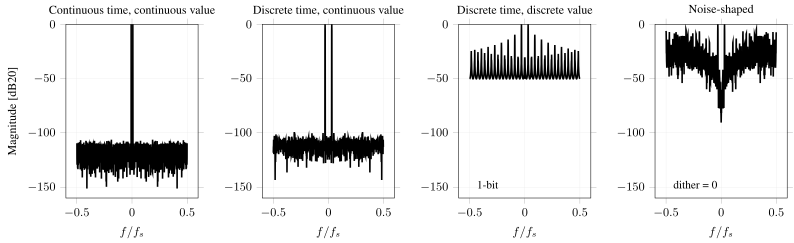
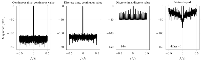
Assume 1-bit quantizer, what would be the maximum ENOB?

OSR	Oversampling	First-order	Second-order
4	2.0	3.1	3.9
64	4.0	9.1	13.9
1024	6.0	15.1	23.9

46

Examples

47

def quantize(v,bits):
    #- 2**bits levels reaching +/-1, so bits=1 is
    #- a genuine two-level quantizer
    levels = 2**bits
    if(levels == 2):
        return 1.0 if v >= 0 else -1.0
    step = 2/(levels-1)
    return float(np.clip(np.round(v/step)*step,-1,1))

# u is discrete time, continuous value input
M = len(u)
y_sd = np.zeros(M)
x = np.zeros(M)
for n in range(1,M):
    x[n] = x[n-1] + (u[n]-y_sd[n-1])
    y_sd[n] = quantize(x[n]
        + dither*np.random.randn()/(4*2**bits),bits)

48

49

50

51

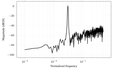
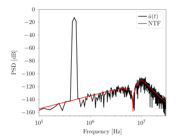
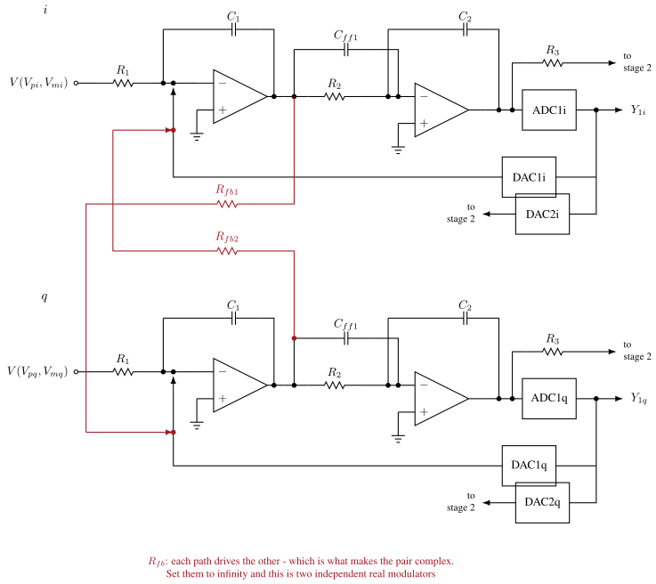
Resonators in Open-Loop Sigma-Delta Modulators [@wulff09]

52

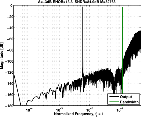
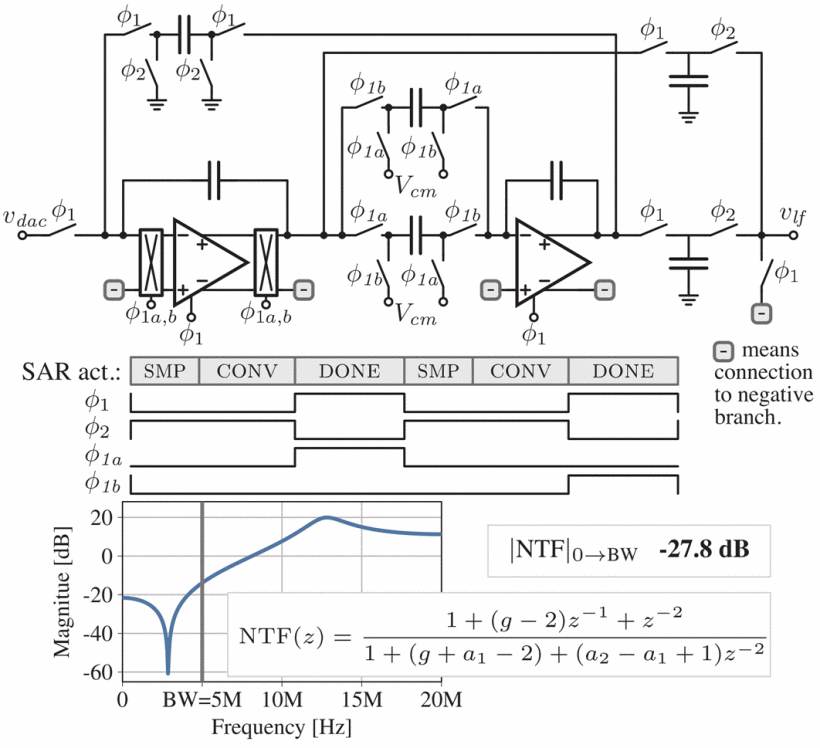
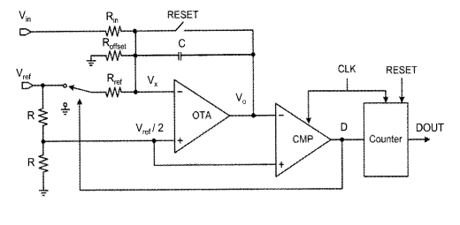
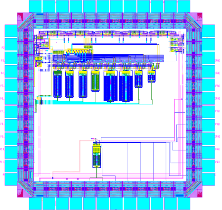
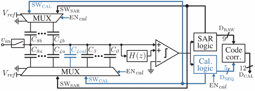
A 68 dB SNDR Compiled Noise-Shaping SAR ADC With On-Chip CDAC Calibration [@garvik19]

53

54

Design Considerations for a Low-Power Control-Bounded A/D Converter

55

56

A 56 mW Continuous-Time Quadrature Cascaded Sigma-Delta Modulator With 77 dB DR in a Near Zero-IF 20 MHz Band

57

Analogue-to-digital converter

58

Summary

One number for an ADC: the figure of merit - Walden for speed-limited, Schreier for noise-limited designs
Ideal quantization gives SQNR = 6.02 N + 1.76 dB, and the white-noise model of it holds only for busy inputs
Oversampling spreads the same noise power over more bandwidth: 3 dB (half a bit) per octave
Feedback around the quantizer shapes the noise away from the band: first-order sigma-delta buys 9 dB per octave, and higher order buys more
The decimation filter is where the promised resolution is actually cashed out
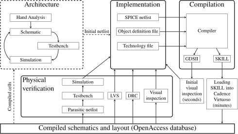
A compiled ADC is a netlist, an object file and a rule file - portable across processes in weeks, and good enough for JSSC

59

Would you like to know more?

60

Thanks!

61