TFE4188 - Lecture 5

Switched-Capacitor Circuits

1

Goal

Understand why we would use switched capacitor circuits

Introduction to discrete-time, and switched capacitor principles and the circuits we need

2

Why

3

Active-RC

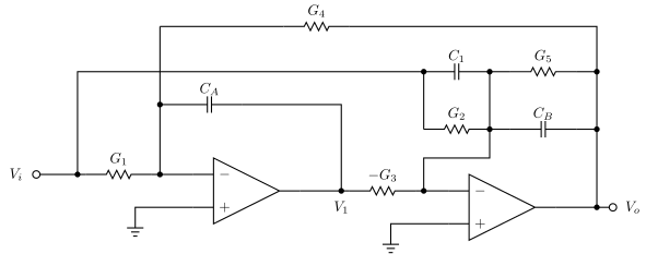
H(s) = \frac{\left[ \frac{C_1}{C_B}s^2 + \frac{G_2}{C_B}s + (\frac{G_1G_3}{C_A C_B})\right]}{\left[ s^2 + \frac{G_5}{C_B}s + \frac{G_3 G_4}{C_A C_B}\right]}

\omega_{p\vert z} \propto \frac{G}{C} = \frac{1}{RC}

4

Gm-C

H(s) = \frac{\left[ s^2\frac{C_X}{C_X + C_B} + s\frac{G_{m5}}{C_X + C_B} + \frac{G_{m2}G_{m4}}{C_A(C_X + C_B)}\right]} {\left[s^2 + s\frac{G_{m3}}{C_X + C_B} + \frac{G_{m1}G_{m2}}{C_A(C_X + C_B)} \right]}

\omega_{p\vert z} \propto \frac{G_m}{C}

5

Switched capacitor

6

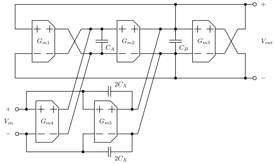
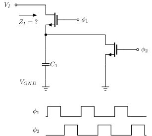
Q_{\phi2\$} = C_1 V_{GND} = 0

Q_{\phi1\$} = C_1 V_{I}

Z_{I} = (V_{I} - V_{GND})/I_{I}

I_{I} = \frac{\Delta Q}{\Delta t} = \left(Q_{\phi1\$} - Q_{\phi2\$}\right) f_{\phi}

Z_{I} = \frac{V_{I} - V_{GND}}{\left(Q_{\phi1\$} - Q_{\phi2\$}\right) f_{\phi}}

Z_{I} = \frac{V_{I}}{\left(C_1 V_{I} - 0 \right) f_{\phi}} = \frac{1}{C_1 f_\phi}

7

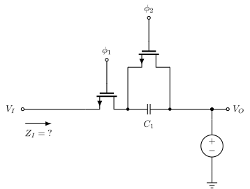
Z_{I} = \frac{V_{I} - V_{O}}{\left(Q_{\phi1\$} - Q_{\phi2\$}\right) f_{\phi}}

Q_{\phi1\$} = C_1 (V_I - V_O)

Q_{\phi2\$} = 0

Z_{I} = \frac{V_{I} - V_{O}}{C_1 \left(V_I - V_O\right) f_{\phi}} = \frac{1}{C_1 f_\phi}

8

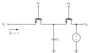
Z_{I} = \frac{ V_{I} - V_{O} }{ \left(Q_{\phi1\$} - Q_{\phi2\$}\right) f_{\phi}}

Q_{\phi1\$} = C_1 V_I

Q_{\phi2\$} = C_1 V_O

Z_{I} = \frac{V_{I} - V_{O}}{\left(C_1 V_I - C_1 V_O\right) f_{\phi}} = \frac{1}{C_1 f_\phi}

9

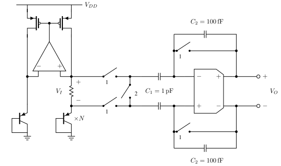
A pipelined 5-Msample/s 9-bit analog-to-digital converter [@Lewis87]

\omega_{p\vert z} \propto f_{clk}\frac{C_1}{C_2}

10

Discrete-Time Signals

11

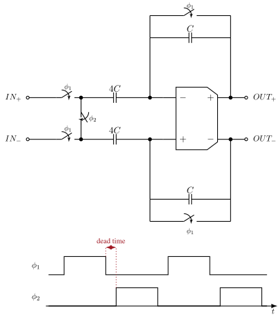
Define \(x_c (t)\) as a continuous time, continuous value signal

Define \(\ell(t) = \begin{cases} 1 & \text{if } t \geq 0 \\ 0 & \text{if } t < 0 \end{cases}\)

Define \(x_{sn}(t) = \frac{x_c(nT)}{\tau}[\ell(t-nT) - \ell(t - nT - \tau)]\)

Define \(x_s(t) = \sum_{n=-\infty}^{\infty}{x_{sn}(t)}\)

Think of a sampled version of an analog signal as an infinite sum of pulse trains where the area under the pulse train is equal to the analog signal.

Why do this?

12

If \(x_s(t) = \sum_{n=-\infty}^{\infty}{x_{sn}(t)}\)

Then \(X_{sn}(s) = \frac{1}{\tau}\frac{1 - e^{-s\tau}}{s} x_c(nT)e^{-snT}\)

And \(X_s(s) = \frac{1}{\tau}\frac{1 - e^{-s\tau}}{s} \sum_{n=-\infty}^{\infty}x_c(nT)e^{-snT}\)

Thus \(\lim_{\tau \to 0} \rightarrow X_s(s) = \sum_{n=-\infty}^{\infty}x_c(nT)e^{-snT}\)

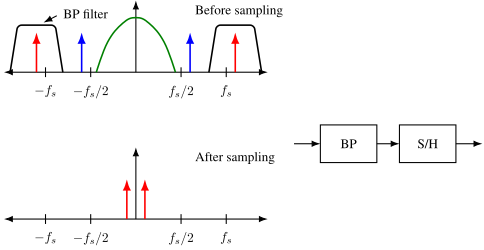
The spectrum of a sampled signal is an infinite sum of frequency shifted spectra

or equivalently

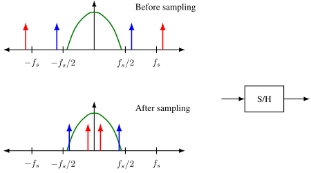
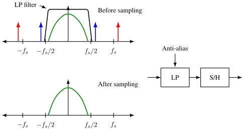
When you sample a signal, then there will be copies of the input spectrum at every \(nf_s\)

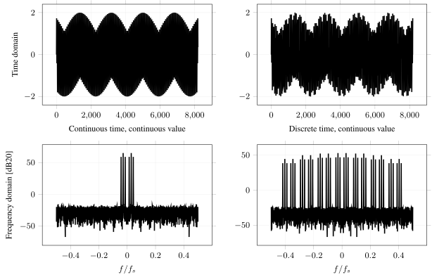
However, if you do an FFT of a sampled signal, then all those infinite spectra will fold down between \(0 \to f_{s1}/2\) or \(- f_{s1}/2 \to f_{s1}/2\) for a complex FFT

13

dt.py - interactive

#- Create a time vector
N = 2**13
t = np.arange(N)

#- Create the "continuous time" signal with multiple 
#- "sinusoidal signals and some noise
#- f1 is deliberately halfway between FFT bins, so the
#- record is not coherent and the window has a job to do
f1 = 233.5/N
fd = 1/N*119
x_s = np.sin(2*np.pi*f1*t) + 1/1024*np.random.randn(N) + \
    0.5*np.sin(2*np.pi*(f1-fd)*t) + 0.5*np.sin(2*np.pi*(f1+fd)*t)

#- Create the sampling vector, and the sampled signal
t_s_unit = [1,1,0,0,0,0,0,0]
t_s = np.tile(t_s_unit,int(N/len(t_s_unit)))
x_sn = x_s*t_s

#- Convert to frequency domain with a hanning window to avoid FFT bin
#- energy spread
Hann = True
if(Hann):
    w = np.hanning(N+1)
else:
    w = np.ones(N+1)
X_s = np.fft.fftshift(np.fft.fft(np.multiply(w[0:N],x_s)))
X_sn = np.fft.fftshift(np.fft.fft(np.multiply(w[0:N],x_sn)))

14

15

16

17

18

X_s(s) = \sum_{n=-\infty}^{\infty}x_c(nT)e^{-snT}

X_s(z) = \sum_{n=-\infty}^{\infty}x_c[n]z^{-n}

For discrete time signal processing we use Z-transform

If you're unfamiliar with the Z-transform, read the book or search https://en.wikipedia.org/wiki/Z-transform

19

Pole-Zero plots

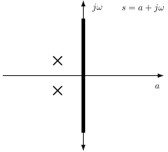
If you're not comfortable with pole/zero plots, have a look at

What does the Laplace Transform really tell us

20

Z-domain

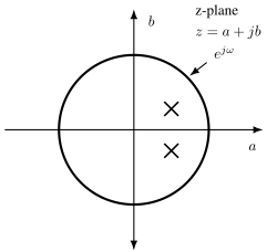
Spectra repeat every \(2\pi\)

Bi-linear transform

s = \frac{2}{T}\frac{z -1}{z + 1}

_{Warning: First-order approximation https://en.wikipedia.org/wiki/Bilinear_transform}

21

First order filter

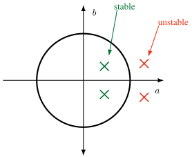
y[n+1] = bx[n] + ay[n] \Rightarrow Y z = b X + a Y

\(y[n] = b x[n-1] + ay[n-1] \Rightarrow Y = b X z^{-1} + a Y z^{-1}\)

H(z) = \frac{b}{z-a}

Infinite-impulse response (IIR)

h[n] = \begin{cases} k & \text{if } n < 1 \\ a^{n-1}b + a^n k & \text{if } n \geq 1 \end{cases}

_{Head's up: Fig 13.12 in AIC is wrong}

22

Second order filter

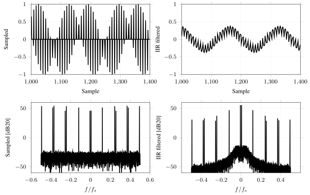
y[n] = b x[n-1] + 2a\, y[n-1] - (a^2 + b^2)\, y[n-2]

H(z) = \frac{b z}{z^2 - 2a z + (a^2+b^2)}

\[z_p = a + jb\]

iir.py - interactive

23

24

Finite-impulse response(FIR)

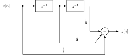
H(z) = \frac{1}{3}\sum_{i=0}^2 z^{-i} = \frac{1}{3}\left(1 + z^{-1} + z^{-2}\right)

25

Switched-Capacitor

26

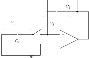
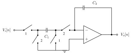
Q_{1\phi_1\$} = C_1 V_1

Q_{2\phi_1\$} = 0

27

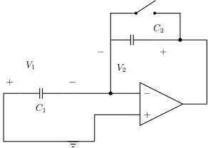
Q_{1\phi_2\$} = 0

Q_{2\phi_2\$} = Q_{1\phi_1\$} = C_1 V_1 = C_2 V_2

\frac{V_2}{V_1} = \frac{C_1}{C_2}

28

Switched capacitor gain circuit

29

30

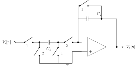
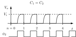
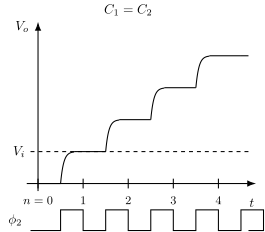
V_o[n+1] = \frac{C_1}{C_2}V_i[n]

V_o z = \frac{C_1}{C_2} V_i

\frac{V_o}{V_i} = H(z) = \frac{C_1}{C_2}z^{-1}

31

Switched capacitor integrator

32

33

V_o[n] = V_o[n-1] + \frac{C_1}{C_2}V_i[n-1]

V_o - z^{-1}V_o = \frac{C_1}{C_2}z^{-1}V_i

H(z) = \frac{C_1}{C_2}\frac{z^{-1}}{1-z^{-1} } = \frac{C_1}{C_2}\frac{1}{z-1}

34

Both phases add noise, \(V_n^2 > \frac{2 k T}{C}\)

35

Mean \(\overline{x(t)} = \lim_{T\to\infty} \frac{1}{T}\int^{+T/2}_{-T/2}{ x(t) dt}\)

Mean Square \(\overline{x^2(t)} = \lim_{T\to\infty} \frac{1}{T}\int^{+T/2}_{-T/2}{ x^2(t) dt}\)

Variance \(\sigma^2 = \overline{x^2(t)} - \overline{x(t)}^2\)

where \(\sigma\) is the standard deviation. If mean is removed, or is zero, then \(\sigma^2 = \overline{x^2(t)}\)

Assume two random processes, \(x_1(t)\) and \(x_2(t)\) with mean of zero (or removed). \(x_{tot}(t) = x_1(t) + x_2(t)\) \(x_{tot}^2(t) = x_1^2(t) + x_2^2(t) + 2x_1(t)x_2(t)\)

Variance (assuming mean of zero) \(\sigma^2_{tot} = \lim_{T\to\infty} \frac{1}{T}\int^{+T/2}_{-T/2}{ x_{tot}^2(t) dt}\) \(\sigma^2_{tot} = \sigma_1^2 + \sigma_2^2 + \lim_{T\to\infty} \frac{1}{T}\int^{+T/2}_{-T/2}{ 2x_1(t)x_2(t) dt}\)

Assuming uncorrelated processes (covariance is zero), then \(\sigma^2_{tot} = \sigma_1^2 + \sigma_2^2\)

36

Sub-circuits for SC-circuits

37

OTA

38

39

40

41

Switches

42

43

44

wulffern/sun_sar9b_sky130nm

45

46

Non-overlapping clocks

47

48

Example

49

50

Summary

A switched capacitor is a resistor R = 1/(f C) made of ratio-accurate parts: SC filters get their time constants from C ratios and a clock
Sampling moves the world to discrete time: the z-domain, aliasing and the sample-rate theorem come with it
The parasitic-insensitive integrator and the SC gain stage are the two workhorse circuits; correlated double sampling throws in offset removal
Every sample costs kT/C of noise - capacitor sizes come from the noise budget, not the layout
Switches need non-overlapping clocks, and bootstrapping when the signal swings
Behind every SC circuit stands an OTA and its bias; the settling budget is half a clock period, verified in the transient

51

Would you like to know more?

52

Thanks!

53